painful truncnorm

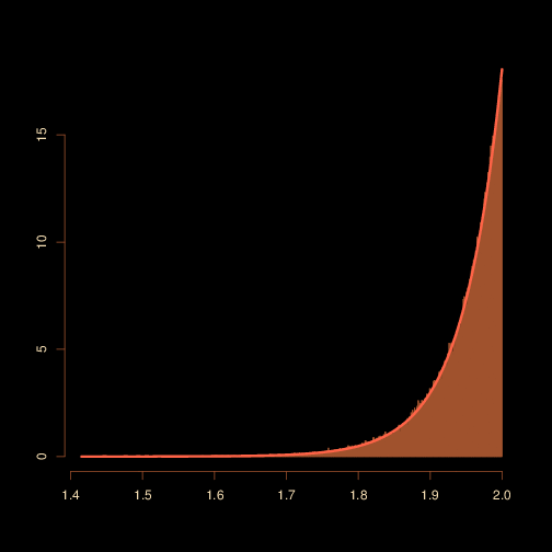As I wanted to simulate truncated normals in a hurry, I coded the inverse cdf approach:

[sourcecode language=”r” gutter=”false”]
truncnorm=function(a,b,mu,sigma){
u=runif(1)
u=qnorm(pnorm((a-mu)/sigma)*(1-u)+u*pnorm((b-mu)/sigma))
return(mu+sigma*u)
}
[/sourcecode]

instead of using my own accept-reject algorithm. Poor shortcut as the method fails when a and b are too far from μ

[sourcecode language=”r” gutter=”false”]
> truncnorm(1,2,3,4)
[1] -0.4912926
> truncnorm(1,2,13,1)
[1] Inf
[/sourcecode]

So I introduced a control (and ended up wasting more time than if I had used my optimised accept-reject version!)

[sourcecode language=”r” gutter=”false”]
truncnorm=function(a,b,mu,sigma){
u=runif(1)
if (pnorm((b-mu)/sigma)-pnorm((a-mu)/sigma)>0){
u=qnorm(pnorm((a-mu)/sigma)*(1-u)+u*pnorm((b-mu)/sigma))
}else{
u=-qnorm(pnorm(-(a-mu)/sigma)*(1-u)-u*pnorm(-(b-mu)/sigma))}
return(mu+sigma*u)
}
[/sourcecode]

As shown by the above, it works, even when a=1, b=2 and μ=20. However, this eventually collapses as well and I ended up installing the msm R package that includes rtnorm, an R function running my accept-reject version. (This package was written by Chris Jackson from the MRC Unit in Cambridge.)

This entry was posted on April 9, 2013 at 12:13 am and is filed under R, Statistics with tags Monte Carlo Statistical Methods, msm package, quantile function, R, rtnorm function, simulation, truncated normal. You can follow any responses to this entry through the RSS 2.0 feed. You can leave a response, or trackback from your own site.

10 Responses to “painful truncnorm”

Tim Says:
June 27, 2016 at 9:11 pm

Next time you can use your algorithm implemented in rtnorm function from extraDistr package (https://github.com/twolodzko/extraDistr/blob/master/src/truncated-normal-distribution.cpp) available on CRAN: https://cran.r-project.org/web/packages/extraDistr/index.html :)

Reply
- xi'an Says:
  June 28, 2016 at 8:45 am
  
  Thank you. Impressive collection of standard and not-so-standard distributions. I should try the package. Soon.
  
  Reply
Joint_p Says:
May 20, 2013 at 8:20 pm

I think your comments swallow pasted code ….

truncnorm=function(a,b,mu,sigma){
u0] = qnorm(pnorm((a-mu)/sigma)*(1-u[foo>0])+u[foo>0]*pnorm((b-mu)/sigma))
u[foo<=0] =-qnorm(pnorm(-(a-mu)/sigma)*(1-u[foo<=0])-u[foo<=0]*pnorm(-(b-mu)/sigma))
return(mu+sigma*u)
}

Reply
- xi'an Says:
  June 28, 2016 at 8:45 am
  
  Indeed they did.
  
  Reply
politicalEconomist Says:
April 9, 2013 at 5:45 pm

The truncnorm package looks a little lighter if all you need is the distribution:
http://cran.r-project.org/web/packages/truncnorm/index.html

Reply
Martyn Says:
April 9, 2013 at 3:07 pm

Inversion is more numerically stable in the tails if you use the argument log.p=TRUE for qnorm and pnorm, and pay attention to whether you are in the upper or lower tail.

truncnorm lower) {
limits <- pnorm(c(lower, upper), mean, sd, log.p = TRUE)
u <- limits[2] – rexp(N) %% (limits[2] – limits[1])
qnorm(u, mean, sd, log.p = TRUE)
}
else {
## Use upper tail
-truncnorm(N, -upper, -lower, -mean, sd)
}
}

Reply
RdR Says:
April 9, 2013 at 9:16 am

Wouldn’t it be quicker to copy and paste the code from “R programs for computing truncated distributions” (Nadarajah and Kotz 2006 Jnl Stat. Soft)? link here: http://www.jstatsoft.org/v16/c02/paper

Reply
- xi'an Says:
  April 9, 2013 at 9:24 am
  
  Very nice paper indeed. However, when I try it in extreme conditions, it fails:
  [sourcecode 1=”gutter=""false""” language=””]
  > rtrunc(1,"norm",a=0,b=1,mean=120,sd=1)
  [1] -Inf
  [/sourcecode]
  while rtnorm (msm) does not:
  [sourcecode 1=”gutter=""false""” language=””]
  > rtnorm(1,mean=120,low=0,upp=1)
  [1] 0.9931963
  [/sourcecode]
  
  Reply
  - Joe Liebig Says:
    May 20, 2013 at 6:17 am
    
    This is also my experience. Rtnorm does a very good job in these extreme cases and it seems to be faster than the inverse CDF method. However, I am missing a Rcpp version of this. I have lots of sampling steps involving truncated Normal that I would like to reprogram using RcppArmadillo… Is there any C implementation of this to build on?
  - Joint_p Says:
    May 20, 2013 at 8:17 pm
    
    Thin slices seem to be a problem for this method:
    
    > truncnorm(8,9,0,1)
    [1] 8.0414
    > truncnorm(8,9,0,1)
    [1] 8.0414
    > truncnorm(8,9,0,1)
    [1] 8.209536
    > truncnorm(8,9,0,1)
    [1] 8.125891
    > truncnorm(8,9,0,1)
    [1] 8.076571
    > truncnorm(8,9,0,1)
    [1] Inf
    
    Compare it:
    
    > sum(is.finite(rtnorm(10000,0,1,8,9)))
    [1] 10000
    
    Ok, so I vectorized the original code from this post and did some investigation:
    
    truncnorm=function(a,b,mu,sigma){
    u0] = qnorm(pnorm((a-mu)/sigma)*(1-u[foo>0])+u[foo>0]*pnorm((b-mu)/sigma))
    u[foo<=0] =-qnorm(pnorm(-(a-mu)/sigma)*(1-u[foo<=0])-u[foo 100000-sum(is.finite(truncnorm(rep(8,100000),rep(9,100000),rep(0,100000),rep(1,100000))))
    [1] 9166
    > system.time(truncnorm(rep(8,100000),rep(9,100000),rep(0,100000),rep(1,100000)))
    user system elapsed
    0.08 0.00 0.08
    > system.time((rtnorm(100000,0,1,8,9)))
    user system elapsed
    0.11 0.03 0.14
    
    Clearly, the iCDF is faster. However, it is quite astonishing how fast the A-R sampler is.

Xi'an's Og