Archive for quantile function

tenets of quantile-based inference in Bayesian models

Posted in Books, Statistics with tags , , , , , , , , , , , , , , on June 8, 2025 by xi'an

This 2023 paper of Perepolkin, Goodrich, and Sahlin vaguely relates to our insufficient Gibbs work in that a Bayesian analysis is conducted based solely on quantile summaries. Except that here the input is the entire cdf, or the—inverse cdf—quantile function, or—its derivative—the quantile density function, instead of the probability density function—used as the likelihood in the posterior. Which is a non-problem from a mathematical perspective since all these functions describe the same probability distribution. Which makes the following quote rather puzzling (in its obviousness).

“We aim to show that the quantile-based Bayesian inference using the intermediate depths leads to the same posterior beliefs as the conventional density-based inference.”

The authors still make a big case of the difference, obviously, to the point of proposing a different notation for Y~F. But using the same symbol f for different densities. The formal expression of the posterior based on the quantile function actually requires the cdf function and the density or the quantile density to be available (at least in a numerical sense), witness eqn (11).

The paper still could hold some interest in its computational component. Relating to ABC, obviously, since distributions defined by quantiles and cdfs often come as benchmarks for ABC, when the associated pdf/likelihood is unavailable. Witness g-and-k distributions (with the caveat MCMC can be implemented in this case). Unfortunately, the paper entirely relies on numerical inversion (with a puzzling comment that MCMC rejection gets higher with numerical inversion, p6). And only mentions ABC in the conclusion, possibly to pacify a referee’s comment. And actually consider that “quantile parameterized quantile distributions don’t lend themselves easily as sampling distributions due to the special nature of their parameterization” (p4). Hence making me wonder at the overall relevance of the entire endeavour….

simple, scalable and accurate posterior interval estimation

Posted in Statistics with tags , , , , , , , on July 6, 2016 by xi'an

“There is a lack of simple and scalable algorithms for uncertainty quantification.”

A paper by Cheng Li , Sanvesh Srivastava, and David Dunson that I had missed and which was pointed out on Andrew’s blog two days ago. As recalled in the very first sentence of the paper, above, the existing scalable MCMC algorithms somewhat fail to account for confidence (credible) intervals. In the sense that handling parallel samples does not naturally produce credible intervals.Since the approach is limited to one-dimensional quantity of interest, ζ=h(θ), the authors of the paper consider the MCMC approximations of the cdf of the said quantity ζ based on the manageable subsets like as many different approximations of the same genuine posterior distribution of that quantity ζ. (Corrected by a power of the likelihood but dependent on the particular subset used for the estimation.) The estimate proposed in the paper is a Wasserstein barycentre of the available estimations, barycentre that is defined as minimising the sum of the Wasserstein distances to all estimates. (Why should this measure be relevant: the different estimates may be of different quality). Interestingly (at least at a computational level), the solution is such that the quantile function of the Wasserstein barycentre is the average of the estimated quantiles functions. (And is there an alternative loss returning the median cdf?) A confidence interval based on the quantile function can then be directly derived. The paper shows that this Wasserstein barycentre converges to the true (marginal) posterior as the sample size m of each sample grows to infinity (and faster than 1/√m), with the strange side-result that the convergence is in 1/√n when the MLE of the global parameter θ is unbiased. Strange to me because unbiasedness is highly dependent on parametrisation while the performances of this estimator should not be, i.e., should be invariant under reparameterisation. Maybe this is due to ζ being a linear transform of θ in the convergence theorem… In any case, I find this question of merging cdf’s from poorly defined approximations to an unknown cdf of the highest interest and look forward any further proposal to this effect!

Nonparametric hierarchical Bayesian quantiles

Posted in Books, Statistics, University life with tags , , , , , , , on June 9, 2016 by xi'an

Luke Bornn, Neal Shephard and Reza Solgi have recently arXived a research report on non-parametric Bayesian quantiles. This work relates to their earlier paper that combines Bayesian inference with moment estimators, in that the quantiles do not define entirely the distribution of the data, which then needs to be completed by Bayesian means. But contrary to this previous paper, it does not require MCMC simulation for distributions defined on a variety as, e.g., a curve.

Here a quantile is defined as minimising an asymmetric absolute risk, i.e., an expected loss. It is therefore a deterministic function of the model parameters for a parametric model and a functional of the model otherwise. And connected to a moment if not a moment per se. In the case of a model with a discrete support, the unconstrained model is parameterised by the probability vector θ and β=t(θ). However, the authors study the opposite approach, namely to set a prior on β, p(β), and then complement this prior with a conditional prior on θ, p(θ|β), the joint prior p(β)p(θ|β) being also the marginal p(θ) because of the deterministic relation. However, I am getting slightly lost in the motivation for the derivation of the conditional when the authors pick an arbitrary prior on θ and use it to derive a conditional on β which, along with an arbitrary (“scientific”) prior on β defines a new prior on θ. This works out in the discrete case because β has a finite support. But it is unclear (to me) why it should work in the continuous case [not covered in the paper].

Getting back to the central idea of defining first the distribution on the quantile β, a further motivation is provided in the hierarchical extension of Section 3, where the same quantile distribution is shared by all individuals (e.g., cricket players) in the population, while the underlying distributions for the individuals are otherwise disconnected and unconstrained. (Obviously, a part of the cricket example went far above my head. But one may always idly wonder why all players should share the same distribution. And about what would happen when imposing no quantile constraint but picking instead a direct hierarchical modelling on the θ’s.) This common distribution on β can then be modelled by a Dirichlet hyperprior.

The paper also contains a section on estimating the entire quantile function, which is a wee paradox in that this function is again a deterministic transform of the original parameter θ, but that the authors use instead pointwise estimation, i.e., for each level τ. I find the exercise furthermore paradoxical in that the hierarchical modelling with a common distribution on the quantile β(τ) only is repeated for each τ but separately, while it should be that the entire parameter should share a common distribution. Given the equivalence between the quantile function and the entire parameter θ.

arbitrary distributions with set correlation

Posted in Books, Kids, pictures, R, Statistics, University life with tags , , , , , , , , , , on May 11, 2015 by xi'an

A question recently posted on X Validated by Antoni Parrelada: given two arbitrary cdfs F and G, how can we simulate a pair (X,Y) with marginals  F and G, and with set correlation ρ? The answer posted by Antoni Parrelada was to reproduce the Gaussian copula solution: produce (X’,Y’) as a Gaussian bivariate vector with correlation ρ and then turn it into (X,Y)=(F⁻¹(Φ(X’)),G⁻¹(Φ(Y’))). Unfortunately, this does not work, because the correlation does not keep under the double transform. The graph above is part of my answer for a χ² and a log-Normal cdf for F amd G: while corr(X’,Y’)=ρ, corr(X,Y) drifts quite a  lot from the diagonal! Actually, by playing long enough with my function

[sourcecode language=”r” gutter=”false”]
tacor=function(rho=0,nsim=1e4,fx=qnorm,fy=qnorm)
{
x1=rnorm(nsim);x2=rnorm(nsim)
coeur=rho
rho2=sqrt(1-rho^2)
for (t in 1:length(rho)){
y=pnorm(cbind(x1,rho[t]*x1+rho2[t]*x2))
coeur[t]=cor(fx(y[,1]),fy(y[,2]))}
return(coeur)
}
[/sourcecode]

Playing further, I managed to get an almost flat correlation graph for the admittedly convoluted call

[sourcecode language=”r” gutter=”false”]
tacor(seq(-1,1,.01),
fx=function(x) qchisq(x^59,df=.01),
fy=function(x) qlogis(x^59))
[/sourcecode]

zerocorNow, the most interesting question is how to produce correlated simulations. A pedestrian way is to start with a copula, e.g. the above Gaussian copula, and to twist the correlation coefficient ρ of the copula until the desired correlation is attained for the transformed pair. That is, to draw the above curve and invert it. (Note that, as clearly exhibited by the graph just above, all desired correlations cannot be achieved for arbitrary cdfs F and G.) This is however very pedestrian and I wonder whether or not there is a generic and somewhat automated solution…

painful truncnorm

Posted in R, Statistics with tags , , , , , , on April 9, 2013 by xi'an

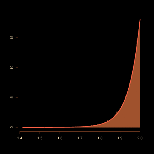
fit of a truncated normal simulation (10⁵ simulations)As I wanted to simulate truncated normals in a hurry, I coded the inverse cdf approach:

[sourcecode language=”r” gutter=”false”]
truncnorm=function(a,b,mu,sigma){
u=runif(1)
u=qnorm(pnorm((a-mu)/sigma)*(1-u)+u*pnorm((b-mu)/sigma))
return(mu+sigma*u)
}
[/sourcecode]

instead of using my own accept-reject algorithm. Poor shortcut as the method fails when a and b are too far from μ

[sourcecode language=”r” gutter=”false”]
> truncnorm(1,2,3,4)
[1] -0.4912926
> truncnorm(1,2,13,1)
[1] Inf
[/sourcecode]

So I introduced a control (and ended up wasting more time than if I had used my optimised accept-reject version!)

[sourcecode language=”r” gutter=”false”]
truncnorm=function(a,b,mu,sigma){
u=runif(1)
if (pnorm((b-mu)/sigma)-pnorm((a-mu)/sigma)>0){
u=qnorm(pnorm((a-mu)/sigma)*(1-u)+u*pnorm((b-mu)/sigma))
}else{
u=-qnorm(pnorm(-(a-mu)/sigma)*(1-u)-u*pnorm(-(b-mu)/sigma))}
return(mu+sigma*u)
}
[/sourcecode]

As shown by the above, it works, even when a=1, b=2 and μ=20. However, this eventually collapses as well and I ended up installing the msm R package that includes rtnorm, an R function running my accept-reject version. (This package was written by Chris Jackson from the MRC Unit in Cambridge.)