Archive for auxiliary variable

Bayesian model comparison with intractable constants

Posted in Books, Kids, pictures, Statistics, Travel, University life with tags , , , , , , , , , , , on February 8, 2016 by xi'an

abcIRichard Everitt, Adam Johansen (Warwick), Ellen Rowing and Melina Evdemon-Hogan have updated [on arXiv] a survey paper on the computation of Bayes factors in the presence of intractable normalising constants. Apparently destined for Statistics and Computing when considering the style. A great entry, in particular for those attending the CRiSM workshop Estimating Constants in a few months!

A question that came to me from reading the introduction to the paper is why a method like Møller et al.’s (2006) auxiliary variable trick should be considered more “exact” than the pseudo-marginal approach of Andrieu and Roberts (2009) since the later can equally be seen as an auxiliary variable approach. The answer was on the next page (!) as it is indeed a special case of Andrieu and Roberts (2009). Murray et al. (2006) also belongs to this group with a product-type importance sampling estimator, based on a sequence of tempered intermediaries… As noted by the authors, there is a whole spectrum of related methods in this area, some of which qualify as exact-approximate, inexact approximate and noisy versions.

Their main argument is to support importance sampling as the method of choice, including sequential Monte Carlo (SMC) for large dimensional parameters. The auxiliary variable of Møller et al.’s (2006) is then part of the importance scheme. In the first toy example, a Poisson is opposed to a Geometric distribution, as in our ABC model choice papers, for which a multiple auxiliary variable approach dominates both ABC and Simon Wood’s synthetic likelihood for a given computing cost. I did not spot which artificial choice was made for the Z(θ)’s in both models, since the constants are entirely known in those densities. A very interesting section of the paper is when envisioning biased approximations to the intractable density. If only because the importance weights are most often biased due to the renormalisation (possibly by resampling). And because the variance derivations are then intractable as well. However, due to this intractability, the paper can only approach the impact of those approximations via empirical experiments. This leads however to the interrogation on how to evaluate the validity of the approximation in settings where truth and even its magnitude are unknown… Cross-validation and bootstrap type evaluations may prove too costly in realistic problems. Using biased solutions thus mostly remains an open problem in my opinion.

The SMC part in the paper is equally interesting if only because it focuses on the data thinning idea studied by Chopin (2002) and many other papers in the recent years. This made me wonder why an alternative relying on a sequence of approximations to the target with tractable normalising constants could not be considered. A whole sequence of auxiliary variable completions sounds highly demanding in terms of computing budget and also requires a corresponding sequence of calibrations. (Now, ABC fares no better since it requires heavy simulations and repeated calibrations, while further exhibiting a damning missing link with the target density. ) Unfortunately, embarking upon a theoretical exploration of the properties of approximate SMC is quite difficult, as shown by the strong assumptions made in the paper to bound the total variation distance to the true target.

love-hate Metropolis algorithm

Posted in Books, pictures, R, Statistics, Travel with tags , , , , , , , , , on January 28, 2016 by xi'an

Hyungsuk Tak, Xiao-Li Meng and David van Dyk just arXived a paper on a multiple choice proposal in Metropolis-Hastings algorithms towards dealing with multimodal targets. Called “A repulsive-attractive Metropolis algorithm for multimodality” [although I wonder why XXL did not jump at the opportunity to use the “love-hate” denomination!]. The proposal distribution includes a [forced] downward Metropolis-Hastings move that uses the inverse of the target density π as its own target, namely 1/{π(x)+ε}. Followed by a [forced] Metropolis-Hastings upward move which target is {π(x)+ε}. The +ε is just there to avoid handling ratios of zeroes (although I wonder why using the convention 0/0=1 would not work). And chosen as 10⁻³²³ by default in connection with R smallest positive number. Whether or not the “downward” move is truly downwards and the “upward” move is truly upwards obviously depends on the generating distribution: I find it rather surprising that the authors consider the same random walk density in both cases as I would have imagined relying on a more dispersed distribution for the downward move in order to reach more easily other modes. For instance, the downward move could have been based on an anti-Langevin proposal, relying on the gradient to proceed further down…

This special choice of a single proposal however simplifies the acceptance ratio (and keeps the overall proposal symmetric). The final acceptance ratio still requires a ratio of intractable normalising constants that the authors bypass by Møller et al. (2006) auxiliary variable trick. While the authors mention the alternative pseudo-marginal approach of Andrieu and Roberts (2009), they do not try to implement it, although this would be straightforward here: since the normalising constants are the probabilities of accepting a downward and an upward move, respectively. Those can easily be evaluated at a cost similar to the use of the auxiliary variables. That is,

– generate a few moves from the current value and record the proportion p of accepted downward moves;
– generate a few moves from the final proposed value and record the proportion q of accepted downward moves;

and replace the ratio of intractable normalising constants with p/q. It is not even clear that one needs those extra moves since the algorithm requires an acceptance in the downward and upward moves, hence generate Geometric variates associated with those probabilities p and q, variates that can be used for estimating them. From a theoretical perspective, I also wonder if forcing the downward and upward moves truly leads to an improved convergence speed. Considering the case when the random walk is poorly calibrated for either the downward or upward move, the number of failed attempts before an acceptance may get beyond the reasonable.

As XXL and David pointed out to me, the unusual aspect of the approach is that here the proposal density is intractable, rather than the target density itself. This makes using Andrieu and Roberts (2009) seemingly less straightforward. However, as I was reminded this afternoon at the statistics and probability seminar in Bristol, the argument for the pseudo-marginal based on an unbiased estimator is that w Q(w|x) has a marginal in x equal to π(x) when the expectation of w is π(x). In thecurrent problem, the proposal in x can extended into a proposal in (x,w), w P(w|x) whose marginal is the proposal on x.

If we complement the target π(x) with the conditional P(w|x), the acceptance probability would then involve

{π(x’) P(w’|x’) / π(x) P(w|x)} / {w’ P(w’|x’) / w P(w|x)} = {π(x’) / π(x)} {w/w’}

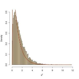
so it seems the pseudo-marginal (or auxiliary variable) argument also extends to the proposal. Here is a short experiment that shows no discrepancy between target and histogram:

[sourcecode language=”r” gutter=”false”]
nozero=1e-300
#love-hate move
move<-function(x){
bacwa=1;prop1=prop2=rnorm(1,x,2)
while (runif(1)>{pi(x)+nozero}/{pi(prop1)+nozero}){
prop1=rnorm(1,x,2);bacwa=bacwa+1}
while (runif(1)>{pi(prop2)+nozero}/{pi(prop1)+nozero})
prop2=rnorm(1,prop1,2)
y=x
if (runif(1)<pi(prop2)*bacwa/pi(x)/fowa){
y=prop2;assign("fowa",bacwa)}
return(y)}
#arbitrary bimodal target
pi<-function(x){.25*dnorm(x)+.75*dnorm(x,mean=5)}
#running the chain
T=1e5
x=5*rnorm(1);luv8=rep(x,T)
fowa=1;prop1=rnorm(1,x,2) #initial estimate
while (runif(1)>{pi(x)+nozero}/{pi(prop1)+nozero}){
fowa=fowa+1;prop1=rnorm(1,x,2)}
for (t in 2:T)
luv8[t]=move(luv8[t-1])
[/sourcecode]

two correlated pseudo-marginals for the price of one!

Posted in Books, Statistics, University life with tags , , , , , , , , , on November 30, 2015 by xi'an

Within two days, two papers on using correlated auxiliary random variables for pseudo-marginal Metropolis-Hastings, one by George Deligiannidis, Arnaud Doucet, Michael Pitt, and Robert Kohn, and another one by Johan Dahlin, Fredrik Lindsten, Joel Kronander, and Thomas Schön! They both make use of the Crank-Nicholson proposal on the auxiliary variables, which is a shrunk Gaussian random walk or an autoregressive model of sorts, and possibly transform these auxiliary variables by inverse cdf or something else.

“Experimentally, the efficiency of computations is increased relative to the standard pseudo-marginal algorithm by up to 180-fold in our simulations.” Deligiannidis et al. 

The first paper by Deligiannidis et al. aims at reducing the variance of the Metropolis-Hastings acceptance ratio by correlating the auxiliary variables. While the auxiliary variable can be of any dimension, all that matters is its transform into a (univariate) estimate of the density, used as pseudo-marginal at each iteration. However, if a Markov kernel is used for proposing new auxiliary variables, the sequence of the pseudo-marginal is no longer a Markov chain. Which implies looking at the auxiliary variables. Nonetheless, they manage to derive a CLT on the log pseudo-marginal estimate, for a latent variable model with sample size growing to infinity. Based on this CLT, they control the correlation in the Crank-Nicholson proposal so that the asymptotic variance  is of order one:  this correlation has to converge to 1 as 1-exp(-χN/T), where N is the number of Monte Carlo samples for T time intervals. Those results extend to the bootstrap particle filter. Upon reflection, it makes much sense aiming for a high correlation since the unbiased estimator of the target hardly changes from one iteration to the next (but needs to move for the method to be validated by Metropolis-Hastings arguments). The two simulation experiments showed massive gains following this scheme, as reported in the above quote.

“[ABC] can be used to approximate the log-likelihood using importance sampling and particle filtering. However, in practice these estimates suffer from a large variance with results in bad mixing for the Markov chain.” Dahlin et al.

In the second paper, which came a day later, presumably induced by the first paper, acknowledged from the start, the authors also make use of the Crank-Nicholson proposal on the auxiliary variables, which is a shrunk Gaussian random walk, and possibly transform these auxiliary variables by inverse cdf or something else. The central part of the paper is about tuning the scale in the Crank-Nicholson proposal, in the spirit of Gelman, Gilks and Roberts (1996). Since all that matters is the (univariate) estimate of the density used as pseudo-marginal, The authors approximate the law of the log-density by a Gaussian distribution, despite the difficulty with the “projected” Markov chain, thus looking for the optimal scaling but only achieving a numerical optimisation rather than the equivalent of the golden number of MCMC acceptance probabilities, 0.234. Although in a sense the above should be the goal for the auxiliary variable acceptance rate, when those are of high enough dimension. One thing I could not find in this paper is how much (generic) improvement is gathered from this modification from an iid version. (Another is linked with the above quote, which I find difficult to understand as ABC is not primarily intended as a pseudo-marginal method. In a sense it is the worst possible pseudo-marginal estimator in that it uses estimators taking values in {0,1}…)

pseudo slice sampling

Posted in Books, Statistics, University life with tags , , , , , on November 26, 2015 by xi'an

The workshop in Warwick last week made me aware of (yet) another arXiv posting I had missed: Pseudo-marginal slice sampling by Iain Murray and Matthew Graham. The idea is to mix the pseudo-marginal approach of Andrieu and Roberts (2009) with a noisy slice sampling scheme à la Neal (2003). The auxiliary random variable u used in the (pseudo-marginal) unbiased estimator of the target I(θ), Î(θ,u), and with distribution q(u) is merged with the random variable of interest so that the joint is

Î(θ,u)q(u)/C

and a Metropolis-Hastings proposal on that target simulating from k(θ,θ’)q(u’) [meaning the auxiliary is simulated independently] recovers the pseudo-marginal Metropolis-Hastings ratio

Î(θ’,u‘)k(θ’,θ)/Î(θ,u)k(θ,θ’)

(which is a nice alternative proof that the method works!). The novel idea in the paper is that the proposal on the auxiliary u can be of a different form, while remaining manageable. For instance, as a two-block Gibbs sampler. Or an elliptical slice sampler for the u component. The argument being that an independent update of u may lead the joint chain to get stuck. Among the illustrations in the paper, an Ising model (with no phase transition issue?) and a Gaussian process applied to the Pima Indian data set (despite a recent prohibition!). From the final discussion, I gather that the modification should be applicable to every (?) case when a pseudo-marginal approach is available, since the auxiliary distribution q(u) is treated as a black box. Quite an interesting read and proposal!

data augmentation with divergence

Posted in Books, Kids, Statistics, University life with tags , , , , , on November 18, 2015 by xi'an

Another (!) Cross Validated question that shed some light on the difficulties of explaining the convergence of MCMC algorithms. Or in understanding conditioning and hierarchical models. The author wanted to know why a data augmentation of his did not converge: In a simplified setting, given an observation y that he wrote as y=h(x,θ), he had built a Gibbs sampler by reconstructing x=g(y,θ) and simulating θ given x: at each iteration t,

  1. compute xt=g(y,θt-1)
  2. simulate θt~π(θ|xt)

and he attributed the lack of convergence to a possible difficulty with the Jacobian. My own interpretation of the issue was rather that condition on the unobserved x was not the same as conditioning on the observed y and hence that y was missing from step 2. And that the simulation of x is useless. Unless one uses it in an augmented scheme à la Xiao-Li… Nonetheless, I like the problem, if only because my very first reaction was to draw a hierarchical dependence graph and to conclude this should be correct, before checking on a toy example that it was not!