Archive for Riemann manifold

comments from Bob

Posted in Books, pictures, Statistics, University life with tags , , , , , , , , , , on April 10, 2026 by xi'an

Bob replied to my short post with further items of information that I find worth sharing:

Thanks for the kind post, Christian. It’s amusing to be the subject of one of these posts given how many of them I’ve read about other people. I really appreciate your summaries. And thanks to everyone in the audience for all the great feedback during and after the talk. Here’s a link to my slides.

One of your students or postdocs mentioned an approach that does continuous adaptation on some kind of polynomial schedule that is provably correct, but I didn’t manage to write down the author/reference or the name of the person who recommended it. If you happen to know what that is, I’d be grateful for the reference.

I would also like to follow up on the Robert & Andrieu paper you mention, but I could not find the exact reference on your Google Scholar page. The closest match I can find is:

Controlled MCMC for optimal sampling. 2001. C Andrieu, CP Robert. INSEE.

Section 1.3 is titled “Criteria for local adaptation.” The section cites two things. The first is Haario et al.’s (1999) sliding window approach, for which HMC moves too fast to be useful locally. The second is the multiple try approach of Liu et al. (2000) and the delayed rejection approach Tierny and Mira (1999). We applied delayed rejection to HMC step size adaptation in a couple of papers before developing GIST (Modi, Barnett and Carpenter in Bayesian Analysis; Turok, Modi, and Carpenter in AISTATS); these mirror our second GIST paper and third GIST paper in doing the step size adaptation for a whole trajectory and at each leapfrog step. The GIST approach is easier to understand, easier to describe mathematically, easier to implement, and is more efficient.

The nice part about GIST compared to Riemannian HMC is that we do not need to do any volume adjustments (which must be autodiffed through), which are cubic, and we do not need an implicit integrator, which is incredibly fussy to tune. The tradeoff is the we require reversibility of the adaptation, which I think is going to be tricky with varying curvature. Of course, we can’t afford to compute Hessian matrices in high dimensions, but we could manage Hessian-vector products if we could figure out how to use just those and we could also manage low-rank plus diagonal approximations or sketches as described in the Nutpie paper.

We’ve arXived the Nutpie paper since the talk:

Preconditioning HMC by minimizing Fisher divergence. arXiv. 2026. Seyboldt, Carlsen, and Carpenter.

The WALNUTS paper has been accepted by JMLR, but currently only the arXiv version is available:

The within-orbit adaptive leapfrog no-U-turn sampler. 2026. Nawaf Bou-Rabee, Bob Carpenter, Tore Selland Kleppe, Sifan Liu. 2025 arXiv; 2026 to appear JMLR.

Working with Nawaf and Tore has made all the difference in the world on this—it’s not something I could have done by myself. Sifan’s the one who came up with the nice characterization of NUTS and Nawaf’s done a number of additional things like providing mixing time bounds for NUTS (with Milo Marsden, who’s sadly no longer with us—he’s gone into finance).

Furthermore, you can adjust the U-turn criterion from 180 degrees to whatever you want to control how much of a full orbit you get. Those tend to be even more wasteful of iterations, though—this is what the plot from the expected integration time of NUTS is supposed to show, but it was confusing in the talk.

The approach you took with Wu Chengye to randomize number of leapfrog steps made a deep impression on me. It’s also wasteful in leapfrog steps because any number of steps greater than or less than about 1/4 of an orbit is wasteful either in computation or because it leads to more diffusive sampling. You can see that it is roughly as gradient efficient as NUTS in a 1000-dimensional standard normal. Interestingly, it’s worse than NUTS for parameter estimates and better for squared parameter estimates, which is overall a win. Nawaf has also published on randomized HMC. I think we could turn down NUTS U-turn criterion below 180 degrees to get something similar with NUTS, but I haven’t tried it.

One important property of your randomized approach is that it is much much easier to code efficiently for GPUs than NUTS, because the conditionals in NUTS are hard to execute in SIMD fashion. There’s a very nice introduction to this problem by Sountsov, Carroll, and Hoffman, in their paper “Running Markov Chain Monte Carlo on Modern Hardware and Software,” which is out on arXiv and also going into the next edition of the Handbook of MCMC). The thing to read about how to code NUTS on GPU is Dance, Glaser, Orbanz, and Adams’s paper, “Efficiently Vectorized MCMC on Modern Accelerators,” which is on arXiv and ICML 2025.

You can also randomize step size to vary the integration time and avoid harmonics, e.g.,

Randomized Hamiltonian Monte Carlo. 2017. Bou-Rabee and Sanz-Serna. Annals of Applied Probability.

thou shalt not slice thine spaghetti

Posted in Statistics with tags , , , , , , , , , , on May 1, 2024 by xi'an

This 2023 work on Slice sampler on manifolds, as presented in the algorithms seminar in Warwick during a recent visit of by Mareike Hasenpflug, consists in designing and validating slice samplers for distributions on manifolds. It is mildly connected to some current work on MCMC algorithms on manifolds through coupling techniques by [my friends & coauthors] Elena Bortolado, Pierre Jacob, and Robin Ryder (who escape temporarily the manifold at each step). As in Neal (2003), uniform draws from the (super)level sets are replaced there with one-step Markov moves within the level set,  that is, slice sampler moves.  The slice sampler actually generalises Neal’s (2003) stepping-out and shrinkage steps rather closely. Based on the standard notion of the Riemannian measure induced by the very structure of the manifold, the model therein assumes that the simulation target is available as a closed-form if unormalised density p(x) against that measure, meaning that problems where the distribution is a push-forward one induced by a mapping onto the manifold are not necessary manageable. The slide sampler is decomposed into choosing (1-dimensional) geodesics defined by the manifold (and generalising great circles), uniformly, and then sampling by this one-dimensional slice sampling over the geodesic, under the level set constraint. Meaning that those geodesics must be manageable enough. (Note that the concept of stepping-out does not mean that the chain ever escapes from the manifold.) Demonstrating the validity and reversibility proves a challenging task.

asymptotically exact inference in likelihood-free models [a reply from the authors]

Posted in R, Statistics with tags , , , , , , , , , , , , , , , , , on December 1, 2016 by xi'an

[Following my post of lastTuesday, Matt Graham commented on the paper with force détails. Here are those comments. A nicer HTML version of the Markdown reply below is also available on Github.]

Thanks for the comments on the paper!

A few additional replies to augment what Amos wrote:

This however sounds somewhat intense in that it involves a quasi-Newton resolution at each step.

The method is definitely computationally expensive. If the constraint function is of the form of a function from an M-dimensional space to an N-dimensional space, with M≥N, for large N the dominant costs at each timestep are usually the constraint Jacobian (∂c/∂u) evaluation (with reverse-mode automatic differentiation this can be evaluated at a cost of O(N) generator / constraint evaluations) and Cholesky decomposition of the Jacobian product (∂c/∂u)(∂c/∂u)‘ with O(N³) cost (though in many cases e.g. i.i.d. or Markovian simulated data, structure in the generator Jacobian can be exploited to give a significantly reduced cost). Each inner Quasi-Newton update involves a pair of triangular solve operations which have a O(N²) cost, two matrix-vector multiplications with O(MN) cost, and a single constraint / generator function evaluation; the number of Quasi-Newton updates required for convergence in the numerical experiments tended to be much less than N hence the Quasi-Newton iteration tended not to be the main cost.

The high computation cost per update is traded off however with often being able to make much larger proposed moves in high-dimensional state spaces with a high chance of acceptance compared to ABC MCMC approaches. Even in the relatively small Lotka-Volterra example we provide which has an input dimension of 104 (four inputs which map to ‘parameters’, and 100 inputs which map to ‘noise’ variables), the ABC MCMC chains using the coarse ABC kernel radius ϵ=100 with comparably very cheap updates were significantly less efficient in terms of effective sample size / computation time than the proposed constrained HMC approach. This was in large part due to the elliptical slice sampling updates in the ABC MCMC chains generally collapsing down to very small moves even for this relatively coarse ϵ. Performance was even worse using non-adaptive ABC MCMC methods and for smaller ϵ, and for higher input dimensions (e.g. using a longer sequence with correspondingly more random inputs) the comparison becomes even more favourable for the constrained HMC approach. Continue reading →

simulation under zero measure constraints [a reply]

Posted in Books, pictures, Statistics, University life with tags , , , , , on November 21, 2016 by xi'an

grahamFollowing my post of last Friday on simulating over zero measure sets, as, e.g., producing a sample with a given maximum likelihood estimator, Dennis Prangle pointed out the recent paper on the topic by Graham and Storkey, and a wee bit later, Matt Graham himself wrote an answer to my X Validated question detailing the resolution of the MLE problem for a Student’s t sample. Including the undoubtedly awesome picture of a 3 observation sample distribution over a non-linear manifold in R³. When reading this description I was then reminded of a discussion I had a few months ago with Gabriel Stolz about his free energy approach that managed the same goal through a Langevin process. Including the book Free Energy Computations he wrote in 2010 with Tony Lelièvre and Mathias Rousset. I now have to dig deeper in these papers, but in the meanwhile let me point out that there is a bounty of 200 points running on this X Validated question for another three days. Offered by Glen B., the #1 contributor to X Validated question for all times.

thermodynamic Monte Carlo

Posted in Books, Statistics, University life with tags , , , , on June 27, 2014 by xi'an

Department of Mathematics and Statistics, University of Warwick

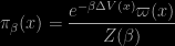
Michael Betancourt, my colleague from Warwick, arXived a month ago a paper about a differential geometry approach to relaxation. (In the Monte Carlo rather than the siesta sense of the term relaxation!) He is considering the best way to link a simple base measure ϖ to a measure of interest π by the sequence

\pi_\beta(x) = \dfrac{e^{-\beta\Delta V(x)}\varpi(x)}{Z(\beta)}

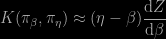
where Z(β) is the normalising constant (or partition function in the  thermodynamic translation). Most methods are highly dependent on how the sequence of β’s is chosen. A first nice result (for me) is that the Kullback-Leibler distance and the partition function are strongly related in that

K(\pi_\beta,\pi_\eta) \approx (\eta-\beta) \dfrac{\text{d}Z}{\text{d}\beta}

which means that the variation in the normalising constant is driving the variation in the Kullback-Leibler distance. The next section goes into differential geometry and the remains from my Master course in differential geometry alas are much too scattered for me to even remember some notions like that of a bundle… So, like Andrew, I have trouble making sense of the resulting algorithm, which updates the temperature β along with the position and speed. (It sounds like an extra and corresponding energy term is added to the original Hamiltonian function.) Even the Beta-Binomial

k|p\sim\mathrm{B}(n,p)\,,\ p\sim\mathrm{Be}(a,b)

example is somewhat too involved for me.  So I tried to write down the algorithm step by step in this special case. Which led to

  1. update β into β-εδp’²
  2. update p into p-εδp’
  3. update p’ into p’+ε{(1-a)/p+(b-1)/(1-p)}
  4. compute the average log-likelihood, λ* under the tempered version of the target (at temperature β)
  5. update p’ into p’+2εβ{(1-a)/p+(b-1)/(1-p)}-ε[λ-λ*]p’
  6. update p’ into p’+ε{(1-a)/p+(b-1)/(1-p)}
  7. update β into β-εδp’²
  8. update p into p-εδp’

where p’ denotes the momentum auxiliary variable associated with the kinetic energy. And λ is the current log-likelihood. (The parameter ε was equal to 0.005 and I could not find the value of δ.) The only costly step in the above list is the approximation of the log-likelihood average λ*. The above details make the algorithm quite clear but I am still missing the intuition behind…