Archive for nested sampling

approximately Bayes [on Skye]

Posted in Mountains, pictures, Running, Statistics, Travel, University life with tags , , , , , , , , , , , , , , , , , , , , , , , , , , , , on May 28, 2026 by xi'an

Wow, what an exciting workshop in an equally exciting place! Strong themes were post-Bayes (Gibbs priors, martingale priors, predictive Bayes, &tc.) and deep neural network modelling. With animated discussions allowed by the free windows planned in the program. And the very early dinner at Sabhal Mòr Ostaig that let a long sunlit evening for impromptu Q&A’s [with a serving of lamb and another of haggis pie!]. Making me realise the large corpus of work I had missed in the past years on these topics, even though the satellite of BayesComp last year was already an eye opener. (Stay tuned for news about BayesComp 2027 & its mirror in Aussois!) The proposal in Jeff Miller’s discussion of Jeremias Knoblauch’s overview of post-Bayes [I’d rather favour another name!]  to consider directly likelihood values as the data was particularly appealing to me, while reminding me of the foundations of nested sampling. (Hopefully, a new perspective on uncertainty assessment for nested sampling is soon to be completed!)

On the non-academic side, the long days in The North helped with my running with above 90km bagged in the week (and no downpour on the runs). But little to my swimming since the water was cold enough to limit my laps to 5mn each time! Paradoxically the worst day was the one I chose for climbing the Inaccessible Pinnacle (as expanded in another ‘Og entry).

multimodal challenges

Posted in Books, Statistics, University life with tags , , , , , , , , , , on April 30, 2026 by xi'an

At the last mostly Monte Carlo seminar, Pierre Monmarché presented a recent work on post-sampling for multimodal targets: while I  consider the main problem in sampling from generic multimodal targets stands with finding the modes, rather than with exploring local aspects or estimating relative weights of said modes, this made me ponder whether or not this could be accelerated by removing chunks of the already explored modes to induce moves elsewhere, which is a form of radical, brute-force, tempering, or of Wang-Landau.  As for the relative weights, a multiple move proposal can be considered, including our folding idea. Or Geyer’s inverse logistic trick. Or the similar mixture trick we used in our Biometrika paper on nested sampling. Pierre’s approach was closer to adaptive importance sampling, with a self-imposed constraint of fixed sample sizes from (approximate) distributions around each of the modes.

deep Bayes factor

Posted in Books, pictures, Statistics, University life with tags , , , , , , , , , , , , , , , , on August 8, 2024 by xi'an

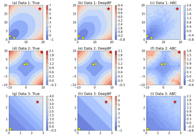
A recently arXived paper proposes an alternative approach to computing Bayes factors via deep learning, Deep Bayes Factors written by Jungeum Kim (presenting her work at JSM this very morning) and Veronika Ročková (whom I have known from her PhD years and whose COPSS Award we very gladly celebrated yesterday!). Which is obviously of interest to me, given my repeated visits to the challenge.

“we introduce Deep Bayes Factor (DeepBF), a neural classifier trained on simulated datasets to learn a mapping whose functional constitutes a Bayes factor estimator.”

Their approach is directly connected with various classification approaches to ABF, incl. the mythical inverse logistic version of Geyer (1994) and noise contrastive estimation of Gutmann and Hyvärinen (2010) (as well as our forested version). Which is called the likelihood-ratio trick here.

“Viewing the Bayes factor through the lens of binary classification aligns with Pudlo et al. (2016), who recast ABC model selection as a classification problem. They employ random forests to select a model by a majority vote. Instead, we focus on binary classification where the purpose is to learn marginal likelihood ratios.  Contrary to the method in Pudlo et al. (2016), our strategy circumvents a secondary learning phase for gauging model posterior estimates, delivering results in only one stage.”

The authors‘ solution stands with learning a classifier from simulated data from both models (and a basic log ratio utility), along iterations updating D from the gradient of the utility, the associated Bayes factor being the ratio D/(1-D) derived from the estimated classifier. There is a cost in producing new samples from the (same) predictives at each iteration (and I wonder if some recycling would be helpful, as well as reducing the sample size for the simpler model). In one of the remarks, the authors point out that “in the effort to see the best ABC performance, we intentionally use the full data Y as a summary statistic”, a remark that I find surprising given the overall consensus that the Bayes factor itself [when based on the full data] is close to optimal.

The method is overall consistent (in the data size n) under classical Bayesian asymptotics, sometimes even when the Bayes factor estimator is inconsistent, naturally expands to pseudo Bayes factors like intrinsic and fractional Bayes factors, also mileage varies in terms of numerical stability.

In the Bayesian model criticism section, the notion of opposing the actual dataset to a simulated one relates very much to Geyer’s (1994) solution. As well as to GANs, as noted in the paper. I did not look closely at the numerical comparisons in the experimental section, but they sound rich enough.

venISBA⁴⁻

Posted in Books, pictures, Statistics, Travel, University life with tags , , , , , , , , , , , , , , , , , , , , , , , on July 8, 2024 by xi'an

As I was released all of a sudden from the Ospedale Civile di Venezia around noon, I managed to attend the last session of ISBA 2024 (after stopping by my airbnb for an emergency coffee next to the hospital and stopping for showering, changing clothes, and eating something more substantial than the contents of IV bags).

My first of these last talks was about coresets by Trevor Campbell, for reducing sample sizes while keeping the likelihood roughly the same (and making me wondering if possibly getting some privacy on the side??) Original algorithm almost completely blind to the data, but a new version by subsample-optimize (KL distance to the posterior) version bringing huge improvements (although I missed the practical details on how the algorithm is reaching this minimum), namely a KL distance of order O(1), i.e., not growing in the sample size. Then, in the same session, a talk by Aikihiko Nakamura on mixing and PDMP, resulting in the novel bouncy Hamiltonian dynamics, which proves time reversible and volume preserving, with no U turns and the time within a given general Hamiltonian value being itself generated w/o rejection. (I am quite sorry to have missed other PDMP talks during the conference, eg, Paul Fearnhead’s, as well as the last poster session…) And I finally jumped rooms to listen to Sam Power on hybrid slice sampling with an MCMC extension to avoid simulating from the Uniform conditional. Reminding me of nested sampling, which also faces this difficulty of sampling from a possibly complex set. This was the end of a wonderful (if shortened by my personal issue) meeting. Next round, see you in Nagoya, Japan (on the Tōkaidō road!).


As a final word about this ISBA 2024 conference in Ca’Foscari, on many levels, I want to most warmly thank my friend Roberto Casarin for his investment and dedication for making the event running so efficiently, in an ideal environment for a meeting of this (800+) size that kept to the Aristotelian unities, especially keeping people together on a unique site without feeling crowded (and very few falling in a Venice canal). And many thanks as well to the local organisers (discounting my nominal inclusion in that group!), the Ca’Foscari staff, and all the students involved in the event!

telescope on evidence for graphical models

Posted in Books, Statistics, University life with tags , , , , , , , , , on February 29, 2024 by xi'an

A recent paper on evidence by Anindya Bhadra, Ksheera Sagar, Sayantan Banerjee (whom I met during Rito’s seminar, since he was also visiting Ismael in Paris, and who mentioned this work), and Jyotishka Datta, on computing the evidence for graphical models. Obtaining an approximation of the evidence attached with a model and a prior on the covariance matrix Ω is a challenge they manage to address in a particularly clever manner.

“the conditional posterior density [of the last column of the covariance matrix] can be evaluated as a product of normal and gamma densities under suitable priors (…) We resolve this [difficulty with the integrated likelihood] by evaluating the required densities in one row or column at a time, and proceeding backwards starting from the p-th row, with appropriate adjustments to Ωp×p at each step via Schur complement. “

Using a telescoping trick, the authors exploit the fact that the decomposition

\log f(y_{1:p})=\log f(y_p|y_{1:p-1},\theta_p)+\log f (y_{1:p-1}|\theta_p)+\log f(\theta_p)-\log f(\theta_p|y_{1:p})

involves a problematic second term that can be ignored by successive cancellations, as shown by Figure 1. The other terms are manageable for some classes of priors on Ω. Like a Wishart. This allows them to call for Chib’s (two-black) method, which requires two independent MCMC runs. Actually, an unfortunate aspect of the approach is that its computational complexity is of order O(M p⁵), where M is the number of MCMC samples, due to the telescopic trick involving calling Chib’s approach for each of the p columns of Ω. While the numerical outcomes compare with nested sampling, annealed importance sampling, and even harmonic mean estimates (!), the computing time usually exceeds those for these other methods, esp. harmonic mean estimates For the specific G-Wishart case, the solution proposed by Atay-Kayis and Massam (2005) proves far superior. Since the main purpose of using evidence is in deriving Bayes factors, I wonder at possible gains in recycling simulations between models, even though this would seem to call for bridge sampling, no considered in the paper.