Archive for posterior predictive

deep Bayes factor

Posted in Books, pictures, Statistics, University life with tags , , , , , , , , , , , , , , , , on August 8, 2024 by xi'an

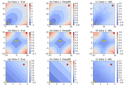
A recently arXived paper proposes an alternative approach to computing Bayes factors via deep learning, Deep Bayes Factors written by Jungeum Kim (presenting her work at JSM this very morning) and Veronika Ročková (whom I have known from her PhD years and whose COPSS Award we very gladly celebrated yesterday!). Which is obviously of interest to me, given my repeated visits to the challenge.

“we introduce Deep Bayes Factor (DeepBF), a neural classifier trained on simulated datasets to learn a mapping whose functional constitutes a Bayes factor estimator.”

Their approach is directly connected with various classification approaches to ABF, incl. the mythical inverse logistic version of Geyer (1994) and noise contrastive estimation of Gutmann and Hyvärinen (2010) (as well as our forested version). Which is called the likelihood-ratio trick here.

“Viewing the Bayes factor through the lens of binary classification aligns with Pudlo et al. (2016), who recast ABC model selection as a classification problem. They employ random forests to select a model by a majority vote. Instead, we focus on binary classification where the purpose is to learn marginal likelihood ratios.  Contrary to the method in Pudlo et al. (2016), our strategy circumvents a secondary learning phase for gauging model posterior estimates, delivering results in only one stage.”

The authors‘ solution stands with learning a classifier from simulated data from both models (and a basic log ratio utility), along iterations updating D from the gradient of the utility, the associated Bayes factor being the ratio D/(1-D) derived from the estimated classifier. There is a cost in producing new samples from the (same) predictives at each iteration (and I wonder if some recycling would be helpful, as well as reducing the sample size for the simpler model). In one of the remarks, the authors point out that “in the effort to see the best ABC performance, we intentionally use the full data Y as a summary statistic”, a remark that I find surprising given the overall consensus that the Bayes factor itself [when based on the full data] is close to optimal.

The method is overall consistent (in the data size n) under classical Bayesian asymptotics, sometimes even when the Bayes factor estimator is inconsistent, naturally expands to pseudo Bayes factors like intrinsic and fractional Bayes factors, also mileage varies in terms of numerical stability.

In the Bayesian model criticism section, the notion of opposing the actual dataset to a simulated one relates very much to Geyer’s (1994) solution. As well as to GANs, as noted in the paper. I did not look closely at the numerical comparisons in the experimental section, but they sound rich enough.

did variational Bayes work?

Posted in Books, Statistics with tags , , , , , , , , , on May 2, 2019 by xi'an

An interesting ICML 2018 paper by Yuling Yao, Aki Vehtari, Daniel Simpson, and Andrew Gelman I missed last summer on [the fairly important issue of] assessing the quality or lack thereof of a variational Bayes approximation. In the sense of being near enough from the true posterior. The criterion that they propose in this paper relates to the Pareto smoothed importance sampling technique discussed in an earlier post and which I remember discussing with Andrew when he visited CREST a few years ago. The truncation of the importance weights of prior x likelihood / VB approximation avoids infinite variance issues but induces an unknown amount of bias. The resulting diagnostic is based on the estimation of the Pareto order k. If the true value of k is less than ½, the variance of the associated Pareto distribution is finite. The paper suggests to conclude at the worth of the variational approximation when the estimate of k is less than 0.7, based on the empirical assessment of the earlier paper. The paper also contains a remark on the poor performances of the generalisation of this method to marginal settings, that is, when the importance weight is the ratio of the true and variational marginals for a sub-vector of interest. I find the counter-performances somewhat worrying in that Rao-Blackwellisation arguments make me prefer marginal ratios to joint ratios. It may however be due to a poor approximation of the marginal ratio that reflects on the approximation and not on the ratio itself. A second proposal in the paper focus on solely the point estimate returned by the variational Bayes approximation. Testing that the posterior predictive is well-calibrated. This is less appealing, especially when the authors point out the “dissadvantage is that this diagnostic does not cover the case where the observed data is not well represented by the model.” In other words, misspecified situations. This potential misspecification could presumably be tested by comparing the Pareto fit based on the actual data with a Pareto fit based on simulated data. Among other deficiencies, they point that this is “a local diagnostic that will not detect unseen modes”. In other words, what you get is what you see.

priors without likelihoods are like sloths without…

Posted in Books, Statistics with tags , , , , , , , , , , , , on September 11, 2017 by xi'an

“The idea of building priors that generate reasonable data may seem like an unusual idea…”

Andrew, Dan, and Michael arXived a opinion piece last week entitled “The prior can generally only be understood in the context of the likelihood”. Which connects to the earlier Read Paper of Gelman and Hennig I discussed last year. I cannot state strong disagreement with the positions taken in this piece, actually, in that I do not think prior distributions ever occur as a given but are rather chosen as a reference measure to probabilise the parameter space and eventually prioritise regions over others. If anything I find myself even further on the prior agnosticism gradation.  (Of course, this lack of disagreement applies to the likelihood understood as a function of both the data and the parameter, rather than of the parameter only, conditional on the data. Priors cannot be depending on the data without incurring disastrous consequences!)

“…it contradicts the conceptual principle that the prior distribution should convey only information that is available before the data have been collected.”

The first example is somewhat disappointing in that it revolves as so many Bayesian textbooks (since Laplace!) around the [sex ratio] Binomial probability parameter and concludes at the strong or long-lasting impact of the Uniform prior. I do not see much of a contradiction between the use of a Uniform prior and the collection of prior information, if only because there is not standardised way to transfer prior information into prior construction. And more fundamentally because a parameter rarely makes sense by itself, alone, without a model that relates it to potential data. As for instance in a regression model. More, following my epiphany of last semester, about the relativity of the prior, I see no damage in the prior being relevant, as I only attach a relative meaning to statements based on the posterior. Rather than trying to limit the impact of a prior, we should rather build assessment tools to measure this impact, for instance by prior predictive simulations. And this is where I come to quite agree with the authors.

“…non-identifiabilities, and near nonidentifiabilites, of complex models can lead to unexpected amounts of weight being given to certain aspects of the prior.”

Another rather straightforward remark is that non-identifiable models see the impact of a prior remain as the sample size grows. And I still see no issue with this fact in a relative approach. When the authors mention (p.7) that purely mathematical priors perform more poorly than weakly informative priors it is hard to see what they mean by this “performance”.

“…judge a prior by examining the data generating processes it favors and disfavors.”

Besides those points, I completely agree with them about the fundamental relevance of the prior as a generative process, only when the likelihood becomes available. And simulatable. (This point is found in many references, including our response to the American Statistician paper Hidden dangers of specifying noninformative priors, with Kaniav Kamary. With the same illustration on a logistic regression.) I also agree to their criticism of the marginal likelihood and Bayes factors as being so strongly impacted by the choice of a prior, if treated as absolute quantities. I also if more reluctantly and somewhat heretically see a point in using the posterior predictive for assessing whether a prior is relevant for the data at hand. At least at a conceptual level. I am however less certain about how to handle improper priors based on their recommendations. In conclusion, it would be great to see one [or more] of the authors at O-Bayes 2017 in Austin as I am sure it would stem nice discussions there! (And by the way I have no prior idea on how to conclude the comparison in the title!)

Goodness-of-fit statistics for ABC

Posted in Books, Statistics, University life with tags , , , , , on February 1, 2016 by xi'an

“Posterior predictive checks are well-suited to Approximate Bayesian Computation”

Louisiane Lemaire and her coauthors from Grenoble have just arXived a new paper on designing a goodness-of-fit statistic from ABC outputs. The statistic is constructed from a comparison between the observed (summary) statistics and replicated summary statistics generated from the posterior predictive distribution. This is a major difference with the standard ABC distance, when the replicated summary statistics are generated from the prior predictive distribution. The core of the paper is about calibrating a posterior predictive p-value derived from this distance, since it is not properly calibrated in the frequentist sense that it is not uniformly distributed “under the null”. A point I discussed in an ‘Og entry about Andrews’ book a few years ago.

The paper opposes the average distance between ABC acceptable summary statistics and the observed realisation to the average distance between ABC posterior predictive simulations of summary statistics and the observed realisation. In the simplest case (e.g., without a post-processing of the summary statistics), the main difference between both average distances is that the summary statistics are used twice in the first version: first to select the acceptable values of the parameters and a second time for the average distance. Which makes it biased downwards. The second version is more computationally demanding, especially when deriving the associated p-value. It however produces a higher power under the alternative. Obviously depending on how the alternative is defined, since goodness-of-fit is only related to the null, i.e., to a specific model.

From a general perspective, I do not completely agree with the conclusions of the paper in that (a) this is a frequentist assessment and partakes in the shortcomings of p-values and (b) the choice of summary statistics has a huge impact on the decision about the fit since hardly varying statistics are more likely to lead to a good fit than appropriately varying ones.

a unified treatment of predictive model comparison

Posted in Books, Statistics, University life with tags , , , , , , , , , on June 16, 2015 by xi'an

“Applying various approximation strategies to the relative predictive performance derived from predictive distributions in frequentist and Bayesian inference yields many of the model comparison techniques ubiquitous in practice, from predictive log loss cross validation to the Bayesian evidence and Bayesian information criteria.”

Michael Betancourt (Warwick) just arXived a paper formalising predictive model comparison in an almost Bourbakian sense! Meaning that he adopts therein a very general representation of the issue, with minimal assumptions on the data generating process (excluding a specific metric and obviously the choice of a testing statistic). He opts for an M-open perspective, meaning that this generating process stands outside the hypothetical statistical model or, in Lindley’s terms, a small world. Within this paradigm, the only way to assess the fit of a model seems to be through the predictive performances of that model. Using for instance an f-divergence like the Kullback-Leibler divergence, based on the true generated process as the reference. I think this however puts a restriction on the choice of small worlds as the probability measure on that small world has to be absolutely continuous wrt the true data generating process for the distance to be finite. While there are arguments in favour of absolutely continuous small worlds, this assumes a knowledge about the true process that we simply cannot gather. Ignoring this difficulty, a relative Kullback-Leibler divergence can be defined in terms of an almost arbitrary reference measure. But as it still relies on the true measure, its evaluation proceeds via cross-validation “tricks” like jackknife and bootstrap. However, on the Bayesian side, using the prior predictive links the Kullback-Leibler divergence with the marginal likelihood. And Michael argues further that the posterior predictive can be seen as the unifying tool behind information criteria like DIC and WAIC (widely applicable information criterion). Which does not convince me towards the utility of those criteria as model selection tools, as there is too much freedom in the way approximations are used and a potential for using the data several times.