Archive for confidence intervals

a lesser-known correlate of the Jeffreys-Lindley paradox (with discussion)

Posted in Books, pictures, Statistics, University life with tags , , , , , , , , , , , , , , , on October 19, 2024 by xi'an

Two UBC faculty, Harlan Campbell and Paul Gustafson, wrote a paper entitled “Defining a Credible Interval Is Not Always Possible with “Point-Null” Priors: A Lesser-Known Correlate of the Jeffreys-Lindley Paradox” in Bayesian Analysis (2024, 19, Number 3, pp. 925–984), which got discussed and presented on the BA webinar yesterday. I missed the call for discussion, on a topic I would have liked very much to discuss and an analysis I strongly disagree with. Fortunately, several of the discussants in the webinar and in the printed version advanced some of my points (as. e.g., Bertrand Clarke in the above slide screen-shot from the on-line video).

I find the paper somewhat missing in linking with the history of the topic, with no mention of Berger & Sellke (1987) that comes as a counterpoint to Casella &—the other—Berger (1987), opposing one sided to two sided tests. Or of matching priors, which connect credible and confidence intervals to higher orders. But the central issue with the apparent contradiction between rejecting the point null hypothesis and returning a credible interval that contains the null is that the construction proceeds from a model averaged posterior. Which fundamentally contradicts the construct of a pair of priors attached with each model towards selecting the fittest one. And requires a far-from-innocent choice of respective prior weights for both models, an ill-defined notion I have repeatedly criticised here and elsewhere. Model averaging clashes with model selection in both decision-theoretic and modelling terms. In model averaging terms, the disappearance of the opposition exhibited by the authors in the predictive distribution, as shown by discussants Held and Pawel, is unsurprising. And makes the spike-and-slab prior far of a necessity. Contrariwise to the model selection case where it proves unavoidable. And for which a merged credible interval does not make sense (to me at least) since it should be constructed once one (and only one) of the two models is chosen. At this point, that the other model ever was considered should not impact subsequent inference. And within that perspective I do not see the relevance of agnostic (ignoring the model choice ation) 5% confidence or credible regions.

“…considers the regime of a fixed true parameter value as n increases [and] of a fixed p-value…” (p928)

With regards with the connection with the Jeffreys-Lindley (or Lindley-Jeffreys) so-called paradox, on which I have already written a lot (or even too much!), many of the earlier objections resurface. Like the measure-theoretic difficulty in including within a continuous interval an atom, i.e., a value with a point mass. Which isolates this atom away from any other value in the interval (and of course creates discontinuities). Or fixing the p-value forever after (when n goes to infinity), as in the graph below (p929). Or treating an improper prior without further caution than with a proper prior. Especially when these are “created” by the decision problem itself.


Estimating means of bounded random variables by betting

Posted in Books, Statistics, University life with tags , , , , , , , , , , , , , , , , , , , , , , , on April 9, 2023 by xi'an

Ian Waudby-Smith and Aaditya Ramdas are presenting next month a Read Paper to the Royal Statistical Society in London on constructing a conservative confidence interval on the mean of a bounded random variable. Here is an extended abstract from within the paper:

For each m ∈ [0, 1], we set up a “fair” multi-round game of statistician
against nature whose payoff rules are such that if the true mean happened
to equal m, then the statistician can neither gain nor lose wealth in
expectation (their wealth in the m-th game is a nonnegative martingale),
but if the mean is not m, then it is possible to bet smartly and make
money. Each round involves the statistician making a bet on the next
observation, nature revealing the observation and giving the appropriate
(positive or negative) payoff to the statistician. The statistician then plays
all these games (one for each m) in parallel, starting each with one unit of
wealth, and possibly using a different, adaptive, betting strategy in each.
The 1 − α confidence set at time t consists of all m 2 [0, 1] such that the
statistician’s money in the corresponding game has not crossed 1/α. The
true mean μ will be in this set with high probability.

I read the paper on the flight back from Venice and was impressed by its universality, especially for a non-asymptotic method, while finding the expository style somewhat unusual for Series B, with notions late into being defined if at all defined. As an aside, I also enjoyed the historical connection to Jean Ville‘s 1939 PhD thesis (examined by Borel, Fréchet—his advisor—and Garnier) on a critical examination of [von Mises’] Kollektive. (The story by Glenn Shafer of Ville’s life till the war is remarkable, with the de Beauvoir-Sartre couple making a surprising and rather unglorious appearance!). Himself inspired by a meeting with Wald while in Berlin. The paper remains quite allusive about Ville‘s contribution, though, while arguing about its advance respective to Ville’s work… The confidence intervals (and sequences) depend on a supermartingale construction of the form

M_t(m):=\prod_{i=1}^t \exp\left\{ \lambda_i(X_i-m)-v_i\psi(\lambda_i)\right\}

which allows for a universal coverage guarantee of the derived intervals (and can optimised in λ). As I am getting confused by that point about the overall purpose of the analysis, besides providing an efficient confidence construction, and am lacking in background about martingales, betting, and sequential testing, I will not contribute to the discussion. Especially since ChatGPT cannot help me much, with its main “criticisms” (which I managed to receive while in Italy, despite the Italian Government banning the chabot!)

However, there are also some potential limitations and challenges to this approach. One limitation is that the accuracy of the method is dependent on the quality of the prior distribution used to set the odds. If the prior distribution is poorly chosen, the resulting estimates may be inaccurate. Additionally, the method may not work well for more complex or high-dimensional problems, where there may not be a clear and intuitive way to set up the betting framework.

and

Another potential consequence is that the use of a betting framework could raise ethical concerns. For example, if the bets are placed on sensitive or controversial topics, such as medical research or political outcomes, there may be concerns about the potential for manipulation or bias in the betting markets. Additionally, the use of betting as a method for scientific or policy decision-making may raise questions about the appropriate role of gambling in these contexts.

being totally off the radar… (No prior involved, no real-life consequence for betting, no gambling.)

error bars [reposted]

Posted in Books, Kids, pictures, Statistics, University life with tags , , , , , on March 3, 2019 by xi'an

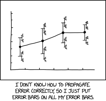
A definitely brilliant entry on xkcd that reflects upon the infinite regress of producing error evaluations that are based on estimates. A must for the next class when I introduce error bars and confidence intervals!

look, look, confidence! [book review]

Posted in Books, Statistics, University life with tags , , , , , , , , , , , , , , , , on April 23, 2018 by xi'an

As it happens, I recently bought [with Amazon Associate earnings] a (used) copy of Confidence, Likelihood, Probability (Statistical Inference with Confidence Distributions), by Tore Schweder and Nils Hjort, to try to understand this confusing notion of confidence distributions. (And hence did not get the book from CUP or anyone else towards purposely writing a review. Or a ½-review like the one below.)

“Fisher squared the circle and obtained a posterior without a prior.” (p.419)

Now that I have gone through a few chapters, I am no less confused about the point of this notion. Which seems to rely on the availability of confidence intervals. Exact or asymptotic ones. The authors plainly recognise (p.61) that a confidence distribution is neither a posterior distribution nor a fiducial distribution, hence cutting off any possible Bayesian usage of the approach. Which seems right in that there is no coherence behind the construct, meaning for instance there is no joint distribution corresponding to the resulting marginals. Or even a specific dominating measure in the parameter space. (Always go looking for the dominating measure!) As usual with frequentist procedures, there is always a feeling of arbitrariness in the resolution, as for instance in the Neyman-Scott problem (p.112) where the profile likelihood and the deviance do not work, but considering directly the distribution of the (inconsistent) MLE of the variance “saves the day”, which sounds a bit like starting from the solution. Another statistical freak, the Fieller-Creasy problem (p.116) remains a freak in this context as it does not seem to allow for a confidence distribution. I also notice an ambivalence in the discourse of the authors of this book, namely that while they claim confidence distributions are both outside a probabilisation of the parameter and inside, “producing distributions for parameters of interest given the data (…) with fewer philosophical and interpretational obstacles” (p.428).

“Bias is particularly difficult to discuss for Bayesian methods, and seems not to be a worry for most Bayesian statisticians.” (p.10)

The discussions as to whether or not confidence distributions form a synthesis of Bayesianism and frequentism always fall short from being convincing, the choice of (or the dependence on) a prior distribution appearing to the authors as a failure of the former approach. Or unnecessarily complicated when there are nuisance parameters. Apparently missing on the (high) degree of subjectivity involved in creating the confidence procedures. Chapter 1 contains a section on “Why not go Bayesian?” that starts from Chris Sims‘ Nobel Lecture on the appeal of Bayesian methods and goes [softly] rampaging through each item. One point (3) is recurrent in many criticisms of B and I always wonder whether or not it is tongue-in-cheek-y… Namely the fact that parameters of a model are rarely if ever stochastic. This is a misrepresentation of the use of prior and posterior distributions [which are in fact] as summaries of information cum uncertainty. About a true fixed parameter. Refusing as does the book to endow posteriors with an epistemic meaning (except for “Bayesian of the Lindley breed” (p.419) is thus most curious. (The debate is repeating in the final(e) chapter as “why the world need not be Bayesian after all”.)

“To obtain frequentist unbiasedness, the Bayesian will have to choose her prior with unbiasedness in mind. Is she then a Bayesian?” (p.430)

A general puzzling feature of the book is that notions are not always immediately defined, but rather discussed and illustrated first. As for instance for the central notion of fiducial probability (Section 1.7, then Chapter 6), maybe because Fisher himself did not have a general principle to advance. The construction of a confidence distribution most often keeps a measure of mystery (and arbitrariness), outside the rather stylised setting of exponential families and sufficient (conditionally so) statistics. (Incidentally, our 2012 ABC survey is [kindly] quoted in relation with approximate sufficiency (p.180), while it does not sound particularly related to this part of the book. Now, is there an ABC version of confidence distributions? Or an ABC derivation?) This is not to imply that the book is uninteresting!, as I found reading it quite entertaining, with many humorous and tongue-in-cheek remarks, like “From Fraser (1961a) and until Fraser (2011), and hopefully even further” (p.92), and great datasets. (Including one entitled Pornoscope, which is about drosophilia mating.) And also datasets with lesser greatness, like the 3000 mink whales that were killed for Example 8.5, where the authors if not the whales “are saved by a large and informative dataset”… (Whaling is a recurrent [national?] theme throughout the book, along with sport statistics usually involving Norway!)

Miscellanea: The interest of the authors in the topic is credited to bowhead whales, more precisely to Adrian Raftery’s geometric merging (or melding) of two priors and to the resulting Borel paradox (xiii). Proposal that I remember Adrian presenting in Luminy, presumably in 1994. Or maybe in Aussois the year after. The book also repeats Don Fraser’s notion that the likelihood is a sufficient statistic, a point that still bothers me. (On the side, I realised while reading Confidence, &tc., that ABC cannot comply with the likelihood principle.) To end up on a French nitpicking note (!), Quenouille is typ(o)ed Quenoille in the main text, the references and the index. (Blame the .bib file!)

X-Outline of a Theory of Statistical Estimation

Posted in Books, Statistics, University life with tags , , , , , , , , , , on March 23, 2017 by xi'an

While visiting Warwick last week, Jean-Michel Marin pointed out and forwarded me this remarkable paper of Jerzy Neyman, published in 1937, and presented to the Royal Society by Harold Jeffreys.

“Leaving apart on one side the practical difficulty of achieving randomness and the meaning of this word when applied to actual experiments…”

“It may be useful to point out that although we are frequently witnessing controversies in which authors try to defend one or another system of the theory of probability as the only legitimate, I am of the opinion that several such theories may be and actually are legitimate, in spite of their occasionally contradicting one another. Each of these theories is based on some system of postulates, and so long as the postulates forming one particular system do not contradict each other and are sufficient to construct a theory, this is as legitimate as any other. “

This paper is fairly long in part because Neyman starts by setting Kolmogorov’s axioms of probability. This is of historical interest but also needed for Neyman to oppose his notion of probability to Jeffreys’ (which is the same from a formal perspective, I believe!). He actually spends a fair chunk on explaining why constants cannot have anything but trivial probability measures. Getting ready to state that an a priori distribution has no meaning (p.343) and that in the rare cases it does it is mostly unknown. While reading the paper, I thought that the distinction was more in terms of frequentist or conditional properties of the estimators, Neyman’s arguments paving the way to his definition of a confidence interval. Assuming repeatability of the experiment under the same conditions and therefore same parameter value (p.344).

“The advantage of the unbiassed [sic] estimates and the justification of their use lies in the fact that in cases frequently met the probability of their differing very much from the estimated parameters is small.”

“…the maximum likelihood estimates appear to be what could be called the best “almost unbiassed [sic]” estimates.”

It is also quite interesting to read that the principle for insisting on unbiasedness is one of producing small errors, because this is not that often the case, as shown by the complete class theorems of Wald (ten years later). And that maximum likelihood is somewhat relegated to a secondary rank, almost unbiased being understood as consistent. A most amusing part of the paper is when Neyman inverts the credible set into a confidence set, that is, turning what is random in a constant and vice-versa. With a justification that the credible interval has zero or one coverage, while the confidence interval has a long-run validity of returning the correct rate of success. What is equally amusing is that the boundaries of a credible interval turn into functions of the sample, hence could be evaluated on a frequentist basis, as done later by Dennis Lindley and others like Welch and Peers, but that Neyman fails to see this and turn the bounds into hard values. For a given sample.

“This, however, is not always the case, and in general there are two or more systems of confidence intervals possible corresponding to the same confidence coefficient α, such that for certain sample points, E’, the intervals in one system are shorter than those in the other, while for some other sample points, E”, the reverse is true.”

The resulting construction of a confidence interval is then awfully convoluted when compared with the derivation of an HPD region, going through regions of acceptance that are the dual of a confidence interval (in the sampling space), while apparently [from my hasty read] missing a rule to order them. And rejecting the notion of a confidence interval being possibly empty, which, while being of practical interest, clashes with its frequentist backup.