Archive for Pareto smoothed importance sampling

Monte Carlo with infinite variances [a surveyal guide]

Posted in Books, Statistics, University life with tags , , , , , , , , , , , , on January 14, 2026 by xi'an

Watch out!, Reiichiro Kawai has just published a survey on infinite variance Monte Carlo methods in Probability Surveys, which is most welcomed as this issue is customarily ignored by both the literature and the practitioners. Radford Neal‘s warning about the dangers of using the harmonic mean estimator of the evidence (as in Newton and Raftery 1996) is an illustration that remains pertinent to this day. In that sense, the survey relates to specific, earlier if recent attempts, such as Chatterjee and Diaconis (2015) or Vehtari et al (2015), with its Pareto correction.

In its recapitulation of the basics of Monte Carlo (closely corresponding to my own introduction of the topic in undergraduate classes), the paper indicates that the consistency of the variance estimator is enough to replace the true variance with its estimator and maintain the CLT. I have often if vaguely wondered at the impact (if any) a variance estimator with (itself) an infinite variance would have. A note to this effect appears at the end of Section 1.2. While being involved from the start, importance sampling has to wait till section 3.2 to be formally introduced. It is also interesting to note that the original result on the optimal importance variance being zero when the integrand is always positive (or negative) is extended here, by noting that a zero variance estimator can always be found by breaking the integrand f into its positive and negative parts, and using now two single samples for the respective integrals. I thus find Example 6 rather unhelpful, even though the entire literature contains such examples with no added value of formal optimal importance samplers. A comment at the end of Example 6 is opens the door to a short discussion of reparametrisation in simulation, a topic rarely discussed in the literature. The use of Rao-Blackwellization as a variance reduction technique that is open to switching from infinite to finite variance, is emphasised as well in Section 2.1.

In relation with a recent musing of mine during a seminar in Warwick, the novel part in the survey on the limited usefulness of control variate is of interest, even though one could predict that linear regression is not doing very well in infinite variance environments. Examples 8 and 9 are most helpful in this respect. It is similarly revealing if unsurprising that basic antithetic variables do not help. The warning about detecting or failing to detect infinite variance situations is well-received.

While theoretically correct, the final section about truncation limit is more exploratory, in that truncation can produce biased answers, whose magnitude is not assessed within the experiment.

finite variance goals

Posted in Books, Statistics, Travel, University life with tags , , , , , , , , , , on November 8, 2025 by xi'an

During Johan Seger’s seminar in Warwick, on the control variate improvements he developed with Rémi Leluc (which PhD thesis committee I joined), Aymeric Dieuleveut, François Portier, and Aigerim Zhuman, I started wondering at whether or not a control variate could turn an infinite variance Monte Carlo estimate into a finite variance one. And asked… ChatGPT about it, with the above reply that is correct if not practical in the least since the example provided therein was reverse-engineering an infinite variance rv into a sum of an infinite variance rv considered as the control variate and a finite variance rv. As summarised below. In practice, this would mean replacing the integrand of interest with a much simpler integrand that shares the same asymptotic behaviour, not an easy task! (As an aside, I found out that enabling MathJax on this ‘Og would cost me $40 a month!)

5. Summary

✅ Theoretical possibility:
Yes — control variates can make an infinite-variance estimator finite, but only if the control’s sample path shares the same tail driver and its expectation is known.infinite variance rv
In real-world Monte Carlo, when X is heavy-tailed, you usually:

  1. Split X = Y + (X-Y), where Y has known expectation and similar tails,

  2. Use Y as control variate, and

  3. Possibly combine with truncation, conditional expectation, or importance sampling for stability.

6th Workshop on Sequential Monte Carlo Methods (#2)

Posted in Mountains, pictures, Running, Statistics, Travel, University life with tags , , , , , , , , , , , , , , , , , , , , , , , on June 5, 2024 by xi'an

Managed to get back from the Pentland hills in time for the Wednesday afternoon session, which proved most interesting as close to my research interests!

Nicola Branchini presented his work with Victor Elvira (a close friend and coauthor, incidentally one of the organisers of the workshop!) on improving self normalised importance sampling by interpreting it as a ratio of estimators based on two samples (which may be the same) and attempting to optimise the joint distribution of said sample. The starting assumption is having (good) marginal importance functions, which means the goal here is in optimising a copula distribution targeting the ratio as quantity of interest. Optimality is however defined in terms of the approximate asymptotic variance of the ratio, which remains an approximation. The idea is nonetheless quite interesting and shows potential for connecting with bridge sampling and… AMIS! As an aside, the talk considered cases when the margins are multivariate, which requires a généralisation of Sklar’s theorem. Simo Särkä then demonstrated how highly parallel processors like GPUs can accommodate Bayesian filters and smoothers in state space models not requiring simulation, gaining a reduction in complexity from O(T) to O(log T). I had not really thought of parallel processing in the recent years, hence was quite pleased at hearing this resolution based on so-called associative scans, and see that implementations were already available in Julia/CUDA.

This was followed by a highly enjoyable poster session, including chats about ABC-SMC for discovery rates, infinite dimensional diffusions, Pareto smoothed importance samplings, &tc with posters by Hugo Marival (coauthor of our importance Monte Carlo recent paper) and Shreya Roy (a student at U of Warwick). With sunny views of Arthur’s Seat (and plenty of people at the top), contrary to the above! Followed by a private party dinner occupying half of a nearby and novel South Indian restaurant that proved quite tasty, local and definitely enjoyable.

For my last morning in town, albeit it was unrelated to the posted abstract, Pierre Del Moral spoke about noisy versions of the ensemble Kalman filter on linear diffusions that allowed for stable solutions under strong enough conditions, encompassing an impressive corpus of work over the past ten years. Alex Beskos presented antithetic multilevel methods for diffusions, which allow to improve the error in the discretisation, even though I did not fully get the whole idea (partly due to dozing out from time to time, a consequence of my last early rounds of Arthur’s Seat in the very early morn).

Daniel Paulin presented a novel unbiased method based on kinetic Langevin dynamics that combines advanced splitting methods with enhanced gradients, avoiding Metropolis correction by coupling and multilevel Monte Carlo approach, achieving unbiasedness by telescoping, but involving an avalanche of acronyms in the leapfrog/Gibbs steps.  And Adam Johansen (U of Warwick) on several recent papers of their divide-and-conquer filtering methods, introduced in a 2017 JCGS paper, following a decomposition of the state variable into low-dimensional components like branches and leaves of a tree.

transport, diffusions, and sampling

Posted in pictures, Statistics, Travel, University life with tags , , , , , , , , , , , , , , , , , , , , , , on November 19, 2022 by xi'an

At the Sampling, Transport, and Diffusions workshop at the Flatiron Institute, on Day #2, Marilou Gabrié (École Polytechnique) gave the second introductory lecture on merging sampling and normalising flows targeting the target distribution, when driven by a divergence criterion like KL, that only requires the shape of the target density. I first wondered about ergodicity guarantees in simultaneous MCMC and map training due to the adaptation of the flow but the update of the map only depends on the current particle cloud in (8). From an MCMC perspective, it sounds somewhat paradoxical to see the independent sampler making such an unexpected come-back when considering that no insider information is available about the (complex) posterior to drive the [what-you-get-is-what-you-see] construction of the transport map. However, the proposed approach superposed local (random-walk like) and global (transport) proposals in Algorithm 1.

Qiang Liu followed on learning transport maps, with the  Interesting notion of causalizing a graph by removing intersections (which are impossible for an ODE, as discussed by Eric Vanden-Eijden’s talk yesterday) through  coupling. Which underlies his notion of rectified flows. Possibly connecting with the next lightning talk by Jonathan Weare on spurious modes created by a variational Monte Carlo sampler and the use of stochastic gradient, corrected by (case-dependent?) regularisation.

Then came a whole series of MCMC talks!

Sam Livingstone spoke on Barker’s proposal (an incoming Biometrika paper!) as part of a general class of transforms g of the MH ratio, using jump processes based on a nasty normalising constant related with g (tractable for the original Barker algorithm). I then realised I had missed his StatSci paper on how to speak to statistical physics researchers!

Charles Margossian spoke about using a massive number of short parallel runs (many-short-chain regime) from a recent paper written with Aki,  Andrew, and Lionel Riou-Durand (Warwick) among others. Which brings us back to the challenge of producing convergence diagnostics and precisely the Gelman-Rubin R statistic or its recent nR avatar (with its linear limitations and dependence on parameterisation, as opposed to fuller distributional criteria). The core of the approach is in using blocks of GPUs to improve and speed-up the estimation of the between-chain variance. (D for R².) I still wonder at a waste of simulations / computing power resulting from stopping the runs almost immediately after warm-up is over, since reaching the stationary regime or an approximation thereof should be exploited more efficiently. (Starting from a minimal discrepancy sample would also improve efficiency.)

Lu Zhang also talked on the issue of cutting down warmup, presenting a paper co-authored with Bob, Andrew, and Aki, recommending Laplace / variational approximations for reaching faster high-posterior-density regions, using an algorithm called Pathfinder that relies on ELBO checks to counter poor performances of Laplace approximations. In the spirit of the workshop, it could be profitable to further transform / push-forward the outcome by a transport map.

Yuling Yao (of stacking and Pareto smoothing fame!) gave an original and challenging (in a positive sense) talk on the many ways of bridging densities [linked with the remark he shared with me the day before] and their statistical significance. Questioning our usual reliance on arithmetic or geometric mixtures. Ignoring computational issues, selecting a bridging pattern sounds not different from choosing a parameterised family of embedding distributions. This new typology of models can then be endowed with properties that are more or less appealing. (Occurences of the Hyvärinen score and our mixtestin perspective in the talk!)

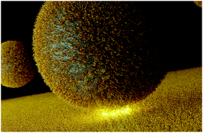
Miranda Holmes-Cerfon talked about MCMC on stratification (illustrated by this beautiful picture of nanoparticle random walks). Which means sampling under varying constraints and dimensions with associated densities under the respective Hausdorff measures. This sounds like a perfect setting for reversible jump and in a sense it is, as mentioned in the talks. Except that the moves between manifolds are driven by the proximity to said manifold, helping with a higher acceptance rate, and making the proposals easier to construct since projections (or the reverses) have a physical meaning. (But I could not tell from the talk why the approach was seemingly escaping the symmetry constraint set by Peter Green’s RJMCMC on the reciprocal moves between two given manifolds).

Conformal Bayesian Computation

Posted in Books, pictures, Statistics, University life with tags , , , , , on July 8, 2021 by xi'an

Edwin Fong and Chris Holmes (Oxford) just wrote a paper on Bayesian scalable methods from a M-open perspective. Borrowing from the conformal prediction framework of Vovk et al. (2005) to achieve frequentist coverage for prediction intervals. The method starts with the choice of a conformity measure that measures how well each observation in the sample agrees with the sample. Which is exchangeable and hence leads to a rank statistic from which a p-value can be derived. Which is the empirical cdf associated with the observed conformities. Following Vovk et al. (2005) and Wasserman (2011) Edwin and Chris note that the Bayesian predictive itself acts like a conformity measure. Predictive that can itself be approximated by MCMC and importance sampling (possibly smoothed by Pareto). The paper also expands the setting to partial exchangeable models, renamed group conformal predictions. While reluctant to engage into turning Bayesian solutions into frequentist ones, I can see some worth in deriving both in order to expose discrepancies and hence signal possible issues with models and priors.