Diego Salmerón and I just arXived a paper on integral priors for multiple model comparison, about deriving reference priors for multiple hypothesis testing. As (so-called) noninformative priors constructed for estimation purposes are usually not appropriate for model selection and testing due to their improperness, Jeffreys-Lindley paradoxes and the like, the methodology of integral priors was developed to get prior distributions for Bayesian model selection when comparing two models, modifying initial improper reference priors. This paper proposes a generalization of this methodology when than two models are to be compared. In order to avoid the above paradoxes and the associated possibility of producing a null recurrent or transient Markov chain, our approach adds an artificial copy of each model under comparison by compactifying the corresponding parametric space and creates an ergodic Markov chain exploring all models that returns the integral priors as marginals of the ergodic and stationary joint distribution. Besides the guarantee of existence of these integral priors and the disappearance of paradoxes that plague estimation reference priors, an additional perk of this methodology is that the simulation of this Markov chain is straightforward as it only requires simulations of imaginary training samples and from the corresponding posterior distributions, for all models, while producing Bayes factor approximations on the side. This renders its implementation automatic and generic, both in the nested and in the nonnested cases. We associated our late friend Juan Antonio Cano to this paper as he was instrumental in initiating both this collaboration and the methodology at its core.
Archive for null recurrence
integral priors for multiple comparison
Posted in Books, Statistics, University life with tags ergodicity, imaginary training sample, improper posteriors, improper priors, intrinsic Bayes factor, Juan Antonio Cano, Markov chain, noninformative priors, null recurrence, pseudo-Bayes factors, reference priors, transience on June 24, 2024 by xi'and≥3 strikes again
Posted in Statistics, University life with tags Boltzmann-Grad limit, Brownian motion, CLT, coupling, Markov process, null recurrence, seminar, Stein effect, transience, University of Bristol, Wiener process on April 23, 2024 by xi'an
Yesterday, Bálint Tóth (University of Bristol and Alfréd Rényi Institute of Mathematics) came to Paris Dauphine for a seminar on the Botlzmann-Grad limit and the existence of a central (double) limit theory. Which was somewhat related with the above video of an earlier seminar, albeit without the first part on the historical roots of the problem. This was a brilliant talk as quite accessible to the entirety of the lab, while providing detailed entries on the mechanism leading to the CLT, in particular the substitution of the physical process by a Markovian(ised) process that stayed closed enough to the original for long enough, a sort of (anti-)coupling idea I had never met before. The other (personally) striking feature of the seminar was the occurrence of the boundary d=3 on the dimension of the process, The same boundary as in the Stein phenomenon (and the difference from recurrent to transient in random walks). But I could not see a clear connection with the present challenge.
null recurrent = zero utility?
Posted in Books, R, Statistics with tags ergodicity, integral priors, Markov chain, Markov kernel, MCMC, null recurrence, R, simulation on April 28, 2022 by xi'an The stability result that the ratio
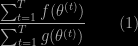
converges holds for a Harris π-null-recurrent Markov chain for all functions f,g in L¹(π) [Meyn & Tweedie, 1993, Theorem 17.3.2] is rather fascinating. However, it is unclear it can be useful in simulation environments, as for the integral priors we have been studying over the years with Juan Antonio Cano and Diego Salmeron Martinez. Above, the result of an experiment where I simulated a Markov chain as a Normal random walk in dimension one, hence a Harris π-null-recurrent Markov chain for the Lebesgue measure λ, and monitored the stabilisation of the ratio (1) when using two densities for f and g, to its expected value (1, shown by a red horizontal line). There is quite a variability in the outcome (repeated 100 times), but the most intriguing is the quick stabilisation of most cumulated averages to values different from 1. Even longer runs display this feature
 which I would blame on the excursions of the random walk far away from the central regions for both f and g, that is on long sequences where zeroes keep being added to numerator and denominators in (1). As far as integral approximation is concerned, this is not very helpful!
Gibbs sampling with incompatible conditionals
Posted in Books, Kids, R, Statistics with tags convergence of Gibbs samplers, cross validated, incompatible conditionals, NAs, null recurrence, R, transience on July 23, 2019 by xi'an An interesting question (with no clear motivation) on X validated wondering why a Gibbs sampler produces NAs… Interesting because multi-layered:
- The attached R code indeed produces NAs because it calls the Negative Binomial Neg(x¹,p) random generator with a zero success parameter, x¹=0, which automatically returns NAs. This can be escaped by returning a one (1) instead.
- The Gibbs sampler is based on a Bin(x²,p) conditional for X¹ and a Neg(x¹,p) conditional for X². When using the most standard version of the Negative Binomial random variate as the number of failures, hence supported on 0,1,2…. these two conditionals are incompatible, i.e., there cannot be a joint distribution behind that returns these as conditionals, which makes the limiting behaviour of the Markov chain harder to study. It however seems to converge to a distribution close to zero, which is not contradictory with the incompatibility property: the stationary joint distribution simply does not enjoy the conditionals used by the Gibbs sampler as its conditionals.
- When using the less standard version of the Negative Binomial random variate understood as a number of attempts for the conditional on X², the two conditionals are compatible and correspond to a joint measure proportional to
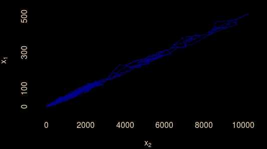
, however this pmf does not sum up to a finite quantity (as in the original Gibbs for Kids example!), hence the resulting Markov chain is at best null recurrent, which seems to be the case for p different from ½. This is unclear to me for p=½.