Archive for bridge sampling

THAMES for mixtures, a reply from the authors

Posted in Books, pictures, R, Statistics, University life with tags , , , , , , , , , , , , , , on June 23, 2025 by xi'an

[Here is a reply to my comments on THAMES sent by the first author of the paper, Martin Metodiev. The above replica of the cover of Rivers of London is obviously unrelated with the reply or the original blog, beyond presenting a fantasy map of the Thames!]

Thank you for your review of our article! Adapting your previous work in this field has been a pleasure. Before I respond to your comments, I would like to emphasize that the simplicity of our estimator lies in its simple analytic expression (a truncated harmonic mean of reciprocal unnormalized posterior density values). Indeed, our package “thamesmix” (recently submitted to CRAN!) has a function to compute the marginal likelihood of any mixture model. This function requires only two parameters: the unnormalized log-posterior function (the logarithm of the prior plus the log-likelihood) and the MCMC simulations from the posterior.

Regarding your main comments:

1. “the evacuation of earlier methods as not simple or not universal enough is rather disingenuous. For instance, software that do not return (latent) allocation vectors can easily be post-processed.”

I could not find an example of post-process simulations on top of MCMC outputs applied to compute these methods. It sounds really interesting, and I would be happy to cite it. Is there a reference that you can recommend?

In any case, the point still stands. Most estimators which we cite with regards to this point do not just need allocation samplers, but also the analytic expressions of the distribution of the allocation vectors or the distribution of the data conditional on these allocation vectors that come with them. I do not think that a closed form of this distribution is available in general.

2.“the handling of the label switching issue—the reason why Larry Wasserman saw mixtures at the same magnitude of evil as tequila!—is problematic for several reasons.”

The fact that our estimator is invariant to label-switching is indeed the core of our method. The simple Gibbs sampler gets stuck in one mode, and this is why the classical version of bridge sampling is biased by a factor of G! in the simulation setting. As you point out, this is successfully resolved when using fully symmetric bridge sampling in the experiment section. However, the computation cost of this fully symmetric estimator rises super-exponentially with G, so I do not see how it could be evaluated for G=15, where the number of symmetric modes is equal to 15! (over one trillion). One of the main points of our article is that the symmetric THAMES can be evaluated in a feasible amount of time, even in such a high-dimensional multivariate setting.

3. “the (legitimate) purpose of using marginal likelihoods for selecting the number G of components is weakened by the intrusion of alternate proposals to assess G from the data”

I would like to point out that these alternate proposals do not in any way impact the definition of the THAMES. It is the simple definition given in Equation (5). They are only used to speed up the computation.

4. “several mentions are made of the other estimators being biased, which is indeed the case for bridge sampling (if not necessarily for importance sampling), but not necessarily a central issue”

The problem that we see with the classical, non-symmetric bridge sampling method in the setting of mixture models is not simply that it is biased. The problem is that the bias is persistent and often roughly equal to the factor of G! when the MCMC sampler failed to switch between modes. We have not had this experience with the THAMES: it converged even when the MCMC was stuck.

easily computed marginal likelihoods for multivariate mixture models using the THAMES estimator

Posted in Books, Statistics, University life with tags , , , , , , , , , , , , , , , , , , , , , on May 25, 2025 by xi'an

Martin Metodiev and his coauthor(es)s have produced another paper on the THAMES Monte Carlo method when specifically targetting marginal likelihoods for mixture models. Since this problem has long been a central interest of mine’s and since the method is closely connected with the harmonic mean solution we developed with Darren Wraith in 2009, (and also included in our 2009 survey with Jean-Michel Marin of evidence approximations, published in Frontiers of Statistical Decision Making and Bayesian Analysis for Jim Berger’s 60th birthday), I quickly went into the paper. The core purpose of this paper is to adapt THAMES to a multimodal setting since using an ellipsoidal region as the support of the Uniform reciprocal importance sampling distribution does not make sense for a multimodal target. After reading it a few times, and while some computational aspects remain obscure to me, I am not convinced this brings an adequate answer to the challenge.  Indeed, while the approach borrows directly from Berkhof et al. (2003) that inspired the resolution we proposed, Jeong (Kate) Lee and myself, the issues I have with the current proposal are that

1. the evacuation of earlier methods as not simple or not universal enough is rather disingenuous. For instance, software that do not return (latent) allocation vectors can easily be post-processed. And the current method uses allocation probabilities just the same (in Section 3.3). Similarly, the random shuffling answer to label (lack of) switching proposed by Sylvia Früwirth-Schnatter—which again can be achieved by post-processing—cannot be rejected on the sole basis that the component means (based on the MCMC sample) are all similar. It is furthermore debatable that the current proposal is simple, when involving relabelling à la Stephens, averaging over permutations, selecting over said permutations by constructing a graph over components (section 3.2.1) and  running a quadratic discriminant analysis (section 3.2.2) on the posterior sample, based on an arbitrary Normal representation of the distributions of the clusters, and finally defining a new ordering constraint (section 3.2.3). Computing efforts  required by the respective methods do not appear in the main text.

2. the handling of the label switching issue—the reason why Larry Wasserman saw mixtures at the same magnitude of evil as tequila!—is problematic for several reasons. My position (since at least 2000!) on the matter is that the proper posterior sample must exhibit label switching and come close to symmetry among the “components”. The label switching problem (section 3.1) is rather when the MCMC sample does not “switch their labels”. The relabelling approach (e.g., à la Stephens) allows for a differentiation between components, to some extent, which helps with computing basic posterior moments for point estimation or for the calibration of the support of the Uniform reciprocal importance sampling distribution, but the use of any relabelling procedure is tampering with the original MCMC sample and thus bound to impact the distribution of the resulting relabelled sample. Furthermore, relabelling depends on the value of G, whereas the actual number of (significant) modes in the posterior is also connected with the (partial) fit of the data to the model, meaning the creation of further modes than those linked with relabelling. Especially when the model is misspecified. Incidentally, the symmetrised version of THAMES (5) does not require relabelling. Neither does the Bayes factor. In addition, the experiment section (4.1.2) mentions that bridge sampling is biased by a factor of G!, which comes as a surprise to me since I associated this factor with the call to Sid Chib’s formula in the absence of label switching, i.e. when the MCMC sample was stuck on a mode, as exposed by Radford Neal in 1999. Is it because bridge sampling is applied to the relabelled sample? It is also surprising that the gap appears in the simulated datasets (Fig.3) and not in the real ones (Fig.5).

3. the (legitimate) purpose of using marginal likelihoods for selecting the number G of components is weakened by the intrusion of alternate proposals to assess G from the data, like the criterion of overlap (section 3.2.1), which instead aims at the number of clusters, with an elimination of “empty components” that should either remain a possibility (within a regular mixture model) or be evacuated with a different modelling (à la Diebolt & Robert, or à la Wasserman). This overlapping criterion is further used in the discriminant analysis that only applies to “non-overlapping components” of the mixture (section 3.2.3)—at which point I got lost in the reordering and simplification of the computation of THAMES (but got reminded of the results of Agostino Nobile in the 2000’s, with whom I used to discuss a lot in my yearly visit to the University of Glasgow).

4. several mentions are made of the other estimators being biased, which is indeed the case for bridge sampling (if not necessarily for importance sampling), but not necessarily a central issue, while the original generalised harmonic proposal by Gelfand and Dey (1994) and thus THAMES produce an unbiased estimator of the inverse of the evidence (thus neither of the evidence nor of the log-evidence). However, in the paper, the volume of the support of the Uniform reciprocal importance sampling distribution is estimated by a basic Monte Carlo coverage probability in (3), which induces the same type of bias as the other methods.

unbiased estimation of a reciprocal

Posted in Books, Statistics, University life with tags , , , , , , , , on November 8, 2024 by xi'an

As often, I came a’X this 2007 paper following an X-validated (if poorly worded) question that linked to it. With weird arguments:

  1. Computing an unbiased estimate of the integral induced by an unnormalised density f is a poor sales argument, as the renormalised object is not a probability density. Call to the unbiased approximation of Bayes factors the paper does not!
  2. The proposed solution involves a replacement of the unnormalised density f  by a substitute and normalised density h  that leads to the identity

\frac{f(y)}{\int f(x)\text dx}=\frac{hf(y)}{1-\int [h(x)-h(y)f(x)/f(x)]\text dx}=\frac{hf(y)}{1-a(y)}

with the assumption that the function a  is between -1 and 1, which requires some insight about the connection between f  and h.

  1. The unbiased estimator is an infinite power series in a(y). Requiring an increasing number of independent generations as the power grows.
  2. The series is unbiasedly terminated by playing roulette (if not Russian roulette!). Stopping when the k-th power estimate is below a certain bound. To be selected with no preliminary knowledge of the range of a.
  3. The uncertainty attached to the power series estimate is not evaluate and could reach the concerning level of an infinite variance.

that may explain for its limited popularity.


Insufficient Gibbs sampling [at COMPSTAT 2024]

Posted in pictures, Statistics, Travel, University life with tags , , , , , , , , , , , , , on August 29, 2024 by xi'an


The COMPSTAT 2024 programme proved somewhat remote from my interests, far from the 1998 version I attended that was buzzing and brimming with MCMC sessions! (Correlatively, apart from the speakers in my own session, I hardly knew anyone there.) I however [missed a Bayesian session as I] attended a session on change-point detection, with a talk by Ziyang Yang (Lancaster University) on an acceleration proposal when the data size is too much, by aggregating similar datapoints, for which I would like to see a theoretical analysis of the impact of this aggregation on the quality (and consistency) of the attached Bayes factor. In my own session, I did not feel overly comfortable with the presentation of a commercial [i.e., for sale] software for pharmacokinetics.

I also enjoyed spending the day in Gießen, from running to the top of nearby Burg Glieberg at sunrise to swimming outdoor in the local 50m Freibad.

deep Bayes factor

Posted in Books, pictures, Statistics, University life with tags , , , , , , , , , , , , , , , , on August 8, 2024 by xi'an

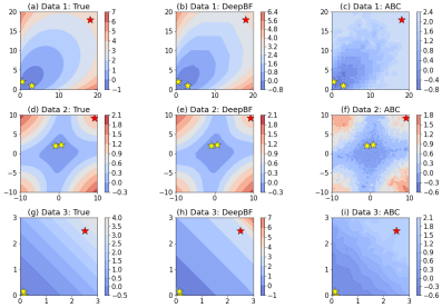
A recently arXived paper proposes an alternative approach to computing Bayes factors via deep learning, Deep Bayes Factors written by Jungeum Kim (presenting her work at JSM this very morning) and Veronika Ročková (whom I have known from her PhD years and whose COPSS Award we very gladly celebrated yesterday!). Which is obviously of interest to me, given my repeated visits to the challenge.

“we introduce Deep Bayes Factor (DeepBF), a neural classifier trained on simulated datasets to learn a mapping whose functional constitutes a Bayes factor estimator.”

Their approach is directly connected with various classification approaches to ABF, incl. the mythical inverse logistic version of Geyer (1994) and noise contrastive estimation of Gutmann and Hyvärinen (2010) (as well as our forested version). Which is called the likelihood-ratio trick here.

“Viewing the Bayes factor through the lens of binary classification aligns with Pudlo et al. (2016), who recast ABC model selection as a classification problem. They employ random forests to select a model by a majority vote. Instead, we focus on binary classification where the purpose is to learn marginal likelihood ratios.  Contrary to the method in Pudlo et al. (2016), our strategy circumvents a secondary learning phase for gauging model posterior estimates, delivering results in only one stage.”

The authors‘ solution stands with learning a classifier from simulated data from both models (and a basic log ratio utility), along iterations updating D from the gradient of the utility, the associated Bayes factor being the ratio D/(1-D) derived from the estimated classifier. There is a cost in producing new samples from the (same) predictives at each iteration (and I wonder if some recycling would be helpful, as well as reducing the sample size for the simpler model). In one of the remarks, the authors point out that “in the effort to see the best ABC performance, we intentionally use the full data Y as a summary statistic”, a remark that I find surprising given the overall consensus that the Bayes factor itself [when based on the full data] is close to optimal.

The method is overall consistent (in the data size n) under classical Bayesian asymptotics, sometimes even when the Bayes factor estimator is inconsistent, naturally expands to pseudo Bayes factors like intrinsic and fractional Bayes factors, also mileage varies in terms of numerical stability.

In the Bayesian model criticism section, the notion of opposing the actual dataset to a simulated one relates very much to Geyer’s (1994) solution. As well as to GANs, as noted in the paper. I did not look closely at the numerical comparisons in the experimental section, but they sound rich enough.