Archive for simulating copulas

Ali–Mikhail–Haq copula, [re]simulated

Posted in Books, R, Statistics with tags , , , , , , , , , on October 13, 2024 by xi'an

When looking for a copula I could simulate from (rather than the Gaussian copula), I found an algorithm for the Ali–Mikhail–Haq copula

C_\theta(u,v) = \frac{uv}{1-\theta(1-u)(1-v)}\quad -1<\theta<1

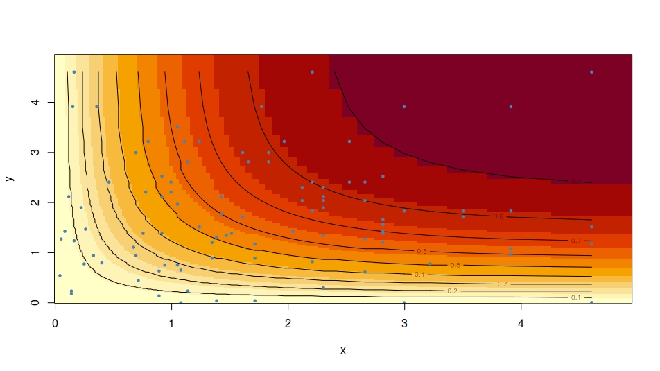
that was proposed by Kumar (2010) as reproduced above. But the method seriously fails in that the range of (U,V) resulting from the simulation does not even cover the (0,1)² square! Unless I made an R coding mistake (which is always a possibility).

sim=function(T=1e3,h=.5){ 
  o=matrix(runif(2*T),T,2)
  a=1-o[,1];b=1-h*(1+2*a*o[,2])+2*h^2*a^2*o[,2]
  d=1+h*(2-4*a+4*a*o[,2])+h^2*(1-4*a*o[,2] +4*a^2*o[,2])
  o[,2]=1-2*o[,2]*(a*h-1)^2/(b+sqrt(d))
  return(o)}

There is no explanation in the paper as to why this algorithm is (not!) working, besides the inverse cdf argument—with the reference in R copBasic temporarily worrying until I checked the cdf inversion is completely numerical—, but a correct version can be derived from inverting the conditional cdf of one component, V, given the other, U. Namely, since the conditional cdf is given by

F(v|U=u) = \frac{v(1-\theta(1-v))}{(1-\theta(1-u)(1-v))^2}

which leads to a second degree polynomial equation (in v) when solving the equation F(v|U=u) = w.

sim=function(T=1e3,h=.5){
  o=matrix(runif(2*T),T,2)
  v1=o[,1];w=o[,2]
  d=(2*h*v1*w-1-h)^2-4*(1-w)*h*(1-h*w*v1^2)
  o[,2]=-2*h*v1*w+1+h-sqrt(d))/(2*h*(1-h*w*v1^2)
  return(1-o)}

And with a more likely outcome (Xed checked by comparing F(u,v) with its empirical version for several pairs (u,v)):

repulsive sampling

Posted in Books, Statistics, University life with tags , , , , , , , , , , , , , , , on January 31, 2024 by xi'an

After a long absence from the monthly Séminaire Parisien de Statistique I attended one today at IHP, including a talk by Diala Hawat on repelled point processes for numerical integration by Hawat et al. The goal is to get (and prove) a universal variance improvement for numerical integration by applying a form of determinantal processes to initial simulations, as eg iid (Poisson process) sampling (without accounting for the O(N²) cost in moving these points). The repelled points are obtain by a single (why single?) move based on a force function (as shown in the slide below), inspired by a Coulomb potential (in the sense that said move appears as one gradient step along the potential). Which reminded me of the pinball sampler, even though the inverse norm was just there to create infinite repulsion near each point. A surprising feature of this repelling step is that it even modifies a (QMC) Sobol process with also an (empirical) improvement in the variance. I wonder if one could construct an MCMC algorithm that would target a joint distribution, maybe via a copula representation, maybe via an equivalent version of HMC.


As an aside, the Bakhvalov results on the existence of a worst case integrand for any deterministic or random sequence (see top slide) made me wonder what the shape of this worst case function is, esp. for a QMC sequence (eg, Sobol). And whether or not they are of any relevance as a counterfactor to the optimal importance functions.

simulating Gumbel’s bivariate exponential distribution

Posted in Books, Kids, R, Statistics with tags , , , , , , , , , , on January 14, 2024 by xi'an

A challenge interesting enough for a sunny New Year morn, found on X validated, namely the simulation of a bivariate exponential distribution proposed by Gumbel in 1960, with density over the positive quadrant in IR²

{}^{ [(\lambda_2+rx_1)(\lambda_1+rx_2)-r]\exp[-(\lambda_1x_1+\lambda_2x_2+rx_1x_2)]}

Although there exists a direct approach based on the fact that the marginals are Exponential distributions and the conditionals signed mixtures of Gamma distributions, an accept-reject algorithm is also available for the pair, with a dominating density representing a genuine mixture of four Gammas, when omitting the X product in the exponential and the negative r in the first term. The efficiency of this accept-reject algorithm is high for r small. However, and in more direct connection with the original question, using this approach to integrate the function equal to the product of the pair, as considered in the original paper of Gumbel, is much less efficient than seeking a quasi-optimal importance function, since this importance function is yet another mixture of four Gammas that produces a much reduced variance at a cheaper cost!

simulating from the joint cdf

Posted in Books, Kids, pictures, R, Statistics, University life with tags , , , , , , , , on July 13, 2022 by xi'an

An X validated question (what else?!) brought back (to me) the question of handling a bivariate cdf for simulation purposes. In the specific case of a copula when thus marginals were (well-)known…. And led me to an erroneous chain of thought, fortunately rescued by Robin Ryder! When the marginal distributions are set, the simulation setup is indeed equivalent to a joint Uniform simulation from a copula

\mathbb P[U_1\leq u_1,U_2\leq u_2,\dots,U_d\leq u_d]=C(u_1,u_2,\dots,u_d)

In specific cases, as for instance the obvious example of Gaussian copulas, there exist customised simulation algorithms. Looking for more generic solutions, I turn to the Bible, where Chapter XI[an], has two entire sections XI.3.2. and XI.3.3 on the topic (even though Luc Devroye does not use the term copula there despite them being introduced in 1959 by A, Sklar, in response to a query of M. Fréchet). In addition to a study of copulas, both sections contain many specific solutions (as for instance in the [unnumbered] Table on page 585) but I found no generic simulation method. My [non-selected] answer to the question was thus to propose standard solutions such as finding one conditional since the marginals are Uniform. Which depends on the tractability of the derivatives of C(·,·).

However, being dissatisfied with this bland answer, I thought further about the problem and came up with a fallacious scheme, namely to first simulate the value p of C(U,V) by drawing a Uniform, and second simulate (U,V) conditional on C(U,V)=p. Going as far as running an R code on a simple copula, as shown above. Fallacious reasoning since (as I knew already!!!), C(U,V) is not uniformly distributed! But has instead a case-dependent distribution… As a (connected) aside, I wonder if the generator attached with Archimedean copulas has any magical feature that help with the generation of the associated copula.

simulating correlated random variables [cont’ed]

Posted in Books, Kids, Statistics with tags , , , , on May 28, 2015 by xi'an

zerocorFollowing a recent post on the topic, and comments ‘Og’s readers kindly provided on that post, the picture is not as clear as I wished it was… Indeed, on the one hand, non-parametric measures of correlation based on ranks are, as pointed out by Clara Grazian and others, invariant under monotonic transforms and hence producing a Gaussian pair or a Uniform pair with the intended rank correlation is sufficient to return a correlated sample for any pair of marginal distributions by the (monotonic) inverse cdf transform.  On the other hand, if correlation is understood as Pearson linear correlation, (a) it is not always defined and (b) there does not seem to be a generic approach to simulate from an arbitrary triplet (F,G,ρ) [assuming the three entries are compatible]. When Kees pointed out Pascal van Kooten‘s solution by permutation, I thought this was a terrific resolution, but after thinking about it a wee bit more, I am afraid it is only an approximation, i.e., a way to return a bivariate sample with a given empirical correlation. Not the theoretical correlation. Obviously, when the sample is very large, this comes as a good approximation. But when facing a request to simulate a single pair (X,Y), this gets inefficient [and still approximate].

Now, if we aim at exact simulation from a bivariate distribution with the arbitrary triplet (F,G,ρ), why can’t we find a generic method?! I think one fundamental if obvious reason is that the question is just ill-posed. Indeed, there are many ways of defining a joint distribution with marginals F and G and with (linear) correlation ρ. One for each copula. The joint could thus be associated with a Gaussian copula, i.e., (X,Y)=(F⁻¹(Φ(A)),G⁻¹(Φ(B))) when (A,B) is a standardised bivariate normal with the proper correlation ρ’. Or it can be associated with the Archimedian copula

C(u; v) = (u-θ + v-θ − 1)-1/θ,

with θ>0 defined by a (linear) correlation of ρ. Or yet with any other copula… Were the joint distribution perfectly well-defined, it would then mean that ρ’ or θ (or whatever natural parameter is used for that copula) do perfectly parametrise this distribution instead of the correlation coefficient ρ. All that remains then is to simulate directly from the copula, maybe a theme for a future post…