
Archive for Bayes factor
on(-line) integral priors for model selection
Posted in Books, Statistics, University life with tags Bayes factor, Bayesian model selection, collaboration, ergodicity, improper priors, integral priors, International Statistical Review, ISI, Juan Antonio Cano, Markov chains, MCMC, noninformative priors, open access, paper, reference priors on February 27, 2026 by xi'an
model uncertainty and missing data: an objective BAyesian perspective
Posted in Books, Statistics, Travel, University life with tags Arnold Zellner, Bayes factor, Bayesian Analysis, Bayesian model comparison, Bayesian predictive, Bayesian variable selection, deviance information criterion, DIC, Don Rubin, Florence Forbes, g-priors, Gilles Celeux, Haar measure, ignorability, improper priors, invariance, Jeffreys priors, linear regression, marginal likelihood, Mike Titterington, missing values, missing-at-random model, model uncertainty, objective Bayes, objective prior distribution, oracle, ozone dataset, reference prior, Rubin’s rules, Spain, time zones, webinar on September 16, 2025 by xi'an My Spanish and objective Bayesian friends Gonzalo García-Donato, María Eugenia Castellanos, Stefano Cabras, Alicia Quirós, and Anabel Forte wrote an fairly exciting paper in BA that is open to discussion (for a few more days), to be discussed on 05 November (4:00 PM UTC | 11:00 AM EST | 5:00 PM CET).
The interplay between missing data and model uncertainty—two classic statistical problems—leads to primary questions that we formally address from an objective Bayesian perspective. For the general regression problem, we discuss the probabilistic justification of Rubin’s rules applied to the usual components of Bayesian variable selection, arguing that prior predictive marginals should be central to the pursued methodology. In the regression settings, we explore the conditions of prior distributions that make the missing data mechanism ignorable, provided that it is missing at random or completely at random. Moreover, when comparing multiple linear models, we provide a complete methodology for dealing with special cases, such as variable selection or uncertainty regarding model errors. In numerous simulation experiments, we demonstrate that our method outperforms or equals others, in consistently producing results close to those obtained using the full dataset. In general, the difference increases with the percentage of missing data and the correlation between the variables used for imputation.
The so-called Rubin’s identity is simply the representation of the posterior probability of a model γ given the observed data x⁰, p(γ|x⁰), as the integrated posterior probability of a model given both observed and latent data, p(γ|x⁰, x¹), against the marginal of latent x¹ given observed x⁰. Since this marginal involves the probabilities p(γ|x⁰), this representation is not directly useful for a numerical implementation.
In this paper, missingness relates to some entries of either the covariates or the response variate. Which is less common but more realistic, especially if some covariates do not contribute to the response. (The missingness mechanism does not matter if the data is missing at random (à la Rubin). The computational solution (p9) is rather standard, simulating the missing variables given the observed variables. In my opinion, the elephant in the room is the super-delicate selection of a prior distribution on the missing covariates, as methinks this impacts in a considerable manner the actual value of the Bayes factor, hence the selection of the surviving model. (As a side remark, we are credited in Celeux et al. (2006) to have “extended DIC for missing data models or when missing data were present”, but our point was instead to point out the arbitrariness of the very definition of DIC in such contexts.)
“The standard Bayesian method for addressing the absence of prior information uses improper distributions. In estimation problems (the model is fixed), the impropriety of priors does not imply any additional difficulty as long as the posterior is proper” (p9)
The authors point out the well-known difficulty with improper priors but still resort to improper priors on the parameters shared by all models—which I dispute as being adequate, despite the arguments put forward on p15, right Haar measure or not—, while sticking to proper priors on the model-dependent parameters. Which unsurprisingly become Zellner’s g-priors. Or rather g’-priors, although the discussion seems to resolve into the (model-free) factor g’ being equal to 1 as for the g-priors. Again a strong term in the derivation of the Bayes factor.
IISA 2024
Posted in Statistics, Travel, University life with tags Bayes factor, Bayesian bootstrap, Bayesian computational methods, Bayesian GANs, Bayesian lasso, Bayesian nonparametrics, betel nut, BNP, Cochin University of Science and Technology, difference in differences model, EM algorithm, IISA 2024, India, insufficient statistic, ISI, Kerala, Kochi, privacy, random walk, Wasserstein distance on January 12, 2025 by xi'an The IISA 2024 conference was held at the Cochin University of Science and Technology (CUSAT), where talks and posters took place. Among the sessions I attended, I attended a talk on colliding random walks that made three or more impossible in the limit, missed the only privacy talk that I could have attended by Vinayak Rao for indulging into a dawnish swimming session in the very decent hotel pool. In the first session I organised, loosely connected with BNP, Antonietta Mira presented a recent work on predicting EU carbon compensation rates, using a information imbalance rank substitute to correlation that could prove quite interesting in privacy settings, albeit no invariant to reparameterisations (with potential connections with Wasserstein distances), Sonia Petrone gave an overview on her substantial amount of work on empirical Bayes in Bayes (EBIB), making me wonder at natural ABC or EM ways to bypass the computation of the empirical Bayes hyperparameter computation (but also on measuring the overfitting degree of EBIB-ing), maybe exploiting the representation of the marginal as an average of predictive, and Debdeep Pati argued towards an interpretable and robust ML, using for estimation divergence a mixture of two KL’s that is remindful of GANs (as well as of Lasso and exponentially tilted empirical likelihood à la Chib & al.), implemented by a form of Bbootstrap. Plus enjoying a locally flavoured acronym, namely BETEL.
 The second session I organised was centred on Bayesian computations, with both Sid Chib and Ritabrata Dutta (U Warwick) presenting a Bayesian modelling of difference-in-difference models in clinical trials and several works on (score based) generalized Bayes models with Shreya Roy (U Warwick), who further won a poster prize at IISA 2024. I terminated the session with a talk on our insufficient Gibbs sampler, which connected with some aspects of both Sid’s and Rito’s talks.

As in earlier editions of IISA I attended, the local organisation was most enjoyable, from supportive staff and students, relaxed atmosphere, easy commutes, heaps of great food, and unlimited chai! Plus meeting and listening to participants I had met in these earlier editions. Looking forward the 2026 edition!
deep Bayes factor
Posted in Books, pictures, Statistics, University life with tags ABC, Bayes factor, Bayesian asymptotics, Bayesian foundations, bridge sampling, Charlie Geyer, classification, COPSS Presidents' Award, Dickey-Savage ratio, fractional Bayes factor, intrinsic Bayes factor, JSM 2024, nested sampling, noise contrasting estimation, Portland, posterior predictive, testing of hypotheses on August 8, 2024 by xi'an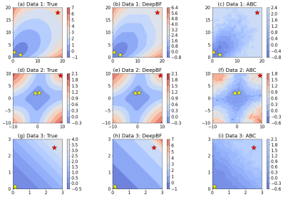 A recently arXived paper proposes an alternative approach to computing Bayes factors via deep learning, Deep Bayes Factors written by Jungeum Kim (presenting her work at JSM this very morning) and Veronika Ročková (whom I have known from her PhD years and whose COPSS Award we very gladly celebrated yesterday!). Which is obviously of interest to me, given my repeated visits to the challenge.
“we introduce Deep Bayes Factor (DeepBF), a neural classifier trained on simulated datasets to learn a mapping whose functional constitutes a Bayes factor estimator.”
Their approach is directly connected with various classification approaches to ABF, incl. the mythical inverse logistic version of Geyer (1994) and noise contrastive estimation of Gutmann and Hyvärinen (2010) (as well as our forested version). Which is called the likelihood-ratio trick here.
“Viewing the Bayes factor through the lens of binary classification aligns with Pudlo et al. (2016), who recast ABC model selection as a classification problem. They employ random forests to select a model by a majority vote. Instead, we focus on binary classification where the purpose is to learn marginal likelihood ratios. Contrary to the method in Pudlo et al. (2016), our strategy circumvents a secondary learning phase for gauging model posterior estimates, delivering results in only one stage.”
The authors‘ solution stands with learning a classifier from simulated data from both models (and a basic log ratio utility), along iterations updating D from the gradient of the utility, the associated Bayes factor being the ratio D/(1-D) derived from the estimated classifier. There is a cost in producing new samples from the (same) predictives at each iteration (and I wonder if some recycling would be helpful, as well as reducing the sample size for the simpler model). In one of the remarks, the authors point out that “in the effort to see the best ABC performance, we intentionally use the full data Y as a summary statistic”, a remark that I find surprising given the overall consensus that the Bayes factor itself [when based on the full data] is close to optimal.
The method is overall consistent (in the data size n) under classical Bayesian asymptotics, sometimes even when the Bayes factor estimator is inconsistent, naturally expands to pseudo Bayes factors like intrinsic and fractional Bayes factors, also mileage varies in terms of numerical stability.
In the Bayesian model criticism section, the notion of opposing the actual dataset to a simulated one relates very much to Geyer’s (1994) solution. As well as to GANs, as noted in the paper. I did not look closely at the numerical comparisons in the experimental section, but they sound rich enough.
insufficient Gibbs sampling bridges as well!
Posted in Books, Kids, pictures, R, Statistics, University life with tags ABC, ABC model choice, Bayes factor, bridge sampling, completion, evidence, Gibbs sampling, insufficient statistic, latent variable, mad, median, model comparison, revision on March 3, 2024 by xi'an
Antoine Luciano, Robin Ryder and I posted a revised version of our insufficient Gibbs sampler on arXiv last week (along with three other revisions or new deposits of mine’s!), following comments and suggestions from referees. Thanks to this revision, we realised that the evidence based on an (insufficient) statistic was also available for approximation by a Monte Carlo estimate attached to the completed sample simulated by the insufficient sampler. Better, a bridge sampling estimator can be used in the same conditions as when the full data is available! In this new version, we thus revisited toy examples first explored in some of my ABC papers on testing (with insufficient statistics), as illustrated by both graphs on this post.


