Archive for Bayesian inference

Bayes in Riddler mode

Posted in Books, Kids, R, Statistics with tags , , , , , on July 7, 2022 by xi'an

A very classical (textbook) question on the Riddler on inferring the contents of an urn from an Hypergeometric experiment:

You have an urn with N  red and white balls, but you have no information about what N might be. You draw n=19 balls at random, without replacement, and you get 8 red balls and 11 white balls. What is your best guess for the original number of balls (red and white) in the urn?

With therefore a likelihood given by

\frac{R!}{(R-8)!}\frac{W!}{(W-11)!}\frac{(R+W-19)!}{(R+W)!}

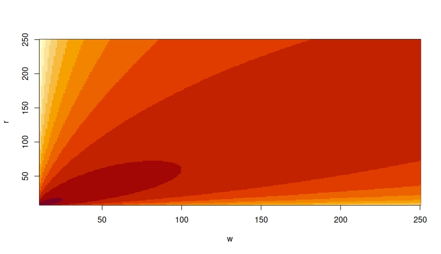
leading to a simple posterior derivation when choosing a 1/RW improper prior. That can be computed for a range of integer values of R and W:

L=function(R,W)lfactorial(R)+lfactorial(W)+
    lfactorial(R+W-19)-lfactorial(R-8)-
    lfactorial(W-11)-lfactorial(R+W)

and produces a posterior mean of 99.1 for R and of 131.2 for W, or a posterior median of 52 for R and 73 for W. And to the above surface for the log-likelihood. Which is unsurprisingly maximal at (8,11). The dependence on the prior is of course significant!

However silly me missed one word in the riddle, namely that R and W were equal… With a proper prior in 1/R², the posterior mean is 42.2 (unstable) and the posterior median 20. While an improper prior in 1/R leads to a posterior mean of 133.7 and a posterior median of 72. However, since the posterior mean increases with the number of values of R for which the posterior is computed, it may be that this mean does not exist!

confidence in confidence

Posted in Statistics, University life with tags , , , , on June 8, 2022 by xi'an

[This is a ghost post that I wrote eons ago and which got lost in the meanwhile.]

Following the false confidence paper, Céline Cunen, Niels Hjort & Tore Schweder wrote a short paper in the same Proceedings A defending confidence distributions. And blame the phenomenon on Bayesian tools, which “might have unfortunate frequentist properties”. Which comes as no surprise since Tore Schweder and Nils Hjort wrote a book promoting confidence distributions for statistical inference.

“…there will never be any false confidence, and we can trust the obtained confidence! “

Their re-analysis of Balch et al (2019) is that using a flat prior on the location (of a satellite) leads to a non-central chi-square distribution as the posterior on the squared distance δ² (between two satellites). Which incidentally happens to be a case pointed out by Jeffreys (1939) against the use of the flat prior as δ² has a constant bias of d (the dimension of the space) plus the non-centrality parameter. And offers a neat contrast between the posterior, with non-central chi-squared cdf with two degrees of freedom

F(\delta)=\Gamma_2(\delta^2/\sigma^2;||y||^2/\sigma^2)

and the confidence “cumulative distribution”

C(\delta)=1-\Gamma_2(|y||^2/\sigma^2;\delta^2/\sigma^2)

Cunen et al (2020) argue that the frequentist properties of the confidence distribution 1-C(R), where R is the impact distance, are robust to an increasing σ when the true value is also R. Which does not seem to demonstrate much. A second illustration of B and C when the distance δ varies and both σ and |y|² are fixed is even more puzzling when the authors criticize the Bayesian credible interval for missing the “true” value of δ, as I find the statement meaningless for a fixed value of |y|²… Looking forward the third round!, i.e. a rebuttal by Balch et al (2019)

Measuring abundance [book review]

Posted in Books, Statistics with tags , , , , , , , , , , , , on January 27, 2022 by xi'an

This 2020 book, Measuring Abundance:  Methods for the Estimation of Population Size and Species Richness was written by Graham Upton, retired professor of applied statistics, for the Data in the Wild series published by Pelagic Publishing, a publishing company based in Exeter.

“Measuring the abundance of individuals and the diversity of species are core components of most ecological research projects and conservation monitoring. This book brings together in one place, for the first time, the methods used to estimate the abundance of individuals in nature.”

Its purpose is to provide a collection of statistical methods for measuring animal abundance or lack thereof. There are four parts: a primer on statistical methods, going no further than maximum likelihood estimation and bootstrap. The term Bayesian only occurs once, in connection with the (a-Bayesian) BIC. (I first spotted a second entry, until I realised this was not a typo and the example truly was about Bawean warty pigs!) The second part is about stationary (or static) individuals, such as trees, and it mostly exposes different recognised ways of sampling, with a focus on minimising the surveyor’s effort. Examples include forestry sampling (with a chainsaw method!) and underwater sampling. There is very little statistics involved in this part apart from the rare appearance of a MLE with an asymptotic confidence interval. There is also very little about misspecified models, except for the occasional warning that the estimates may prove completely wrong. The third part is about mobile individuals, with capture-recapture methods receiving the lion’s share (!). No lion was actually involved in the studies used as examples (but there were grizzly bears from Yellowstone and Banff National Parks). Given the huge variety of capture-recapture models, very little input is found within the book as the practical aspects are delegated to R software like the RMark and mra packages. Very little is written on using covariates or spatial features in such models, mostly dedicated to printed output from R packages with AIC as the sole standard for comparing models. I did not know of distance methods (Chapter 8), which are less invasive counting methods. They however seem to rely on a particular model of missing on individuals as the distance increases. The last section is about estimating the number of species. With again a model assumption that may prove wrong. With the inclusion of diversity measures,

The contents of the book are really down to earth and intended for field data gatherers. For instance, “drive slowly and steadily at 20 mph with headlights and hazard lights on ” (p.91) or “Before starting to record, allow fish time to acclimatize to the presence of divers” (p.91). It is unclear to me how useful the book would prove to be for general statisticians, apart from revealing the huge diversity of methods actually employed in the field. To either build upon these or expose students to their reassessment. More advanced books are McCrea and Morgan (2014), Buckland et al. (2016) and the most recent Seber and Schofield (2019).

[Disclaimer about potential self-plagiarism: this post or an edited version will eventually appear in my Book Review section in CHANCE.]
flow contrastive estimation

Posted in Books, Statistics with tags , , , , , , , , on March 15, 2021 by xi'an

On the flight back from Montpellier, last week, I read a 2019 paper by Gao et al. revisiting the MLE estimation of a parametric family parameter when the normalising constant Z=Z(θ) is unknown. Via noise-contrastive estimation à la Guttman & Hyvärinnen (or à la Charlie Geyer). Treating the normalising constant Z as an extra parameter (as in Kong et al.) and the classification probability as an objective function and calling it a likelihood, which it is not in my opinion as (i) the allocation to the groups is not random and (ii) the original density of the actual observations does not appear in the so-called likelihood.

“When q appears on the right of KL-divergence [against p],  it is forced to cover most of the modes of p, When q appears on the left of KL-divergence, it tends to chase the major modes of p while ignoring the minor modes.”

The flow in the title indicates that the contrastive distribution q is estimated by a flow-based estimator, namely the transform of a basic noise distribution via easily invertible and differentiable transforms, for instance with lower triangular Jacobians. This flow is also estimated directly from the data but the authors complain this estimation is not good enough for noise contrastive estimation and suggest instead resorting to a GAN version where the classification log-probability is maximised in the model parameters and minimsed in the flow parameters. Except that I feel it misses the true likelihood part. In other words, why on Hyperion would estimating all θ, Z=Z(θ), and α at once improve the estimation of Z?

The other aspect that puzzles me is that (12) uses integrated classification probabilities (with the unknown Z as extra parameter), rather than conditioning on the data, Bayes-like. (The difference between (12) and GAN is that here the discriminator function is constrained.) Esp. when the first expectation is replaced with its empirical version.

marginal likelihood as exhaustive X validation

Posted in Statistics with tags , , , , , , , , on October 9, 2020 by xi'an

In the June issue of Biometrika (for which I am deputy editor) Edwin Fong and Chris Holmes have a short paper (that I did not process!) on the validation of the marginal likelihood as the unique coherent updating rule. Marginal in the general sense of Bissiri et al. (2016). Coherent in the sense of being invariant to the order of input of exchangeable data, if in a somewhat self-defining version (Definition 1). As a consequence, marginal likelihood arises as the unique prequential scoring rule under coherent belief updating in the Bayesian framework. (It is unique given the prior or its generalisation, obviously.)

“…we see that 10% of terms contributing to the marginal likelihood come from out-of-sample predictions, using on average less than 5% of the available training data.”

The paper also contains the interesting remark that the log marginal likelihood is the average leave-p-out X-validation score, across all values of p. Which shows that, provided the marginal can be approximated, the X validation assessment is feasible. Which leads to a highly relevant (imho) spotlight on how this expresses the (deadly) impact of the prior selection on the numerical value of the marginal likelihood. Leaving outsome of the least informative terms in the X-validation leads to exactly the log geometric intrinsic Bayes factor of Berger & Pericchi (1996). Most interesting connection with the Bayes factor community but one that depends on the choice of the dismissed fraction of p‘s.
