Archive for Introducing Monte Carlo Methods with R

Short review of the R book

Posted in Books, R, Statistics, University life with tags , , on January 6, 2011 by xi'an

David Scott wrote a review of Introducing Monte Carlo Methods with R in the International Statistical Review that is rather negative, since the main bulk reads as follows:

I found some aspects of the book very disappointing. The first chapter (“Basic R Programming”) has some unfortunate mistakes and some statements, which are contentious at least (“An older assignment operator is <- . . . but it should be ignored for cleaner programming”). The graphs throughout the book appear to be bitmaps—they are quite blurred. Either postscript or pdf graphs should have been produced which would have immeasurably improved the presentation. The book is not an easy read, requiring considerable background to be understood. I found the chapters on MCMC easier than the chapters on general Monte Carlo methods because I had a reasonable understanding of the theory beforehand. There are exercises within and at the end  of all chapters, which appear to be fairly challenging, with the possible exception of the first two chapters.

As undoubtedly obvious to regular readers of the ‘Og, there are certainly many typos found throughout of the book and Chapter 1 is no exception. (The point about using “<-” versus “=” assignment operator is subject to many discussions and I should not have used “older”, even though I strongly dislike the “<-” operator!) David Scott is completely right in complaining about the quality of the graphs, in that the jpeg versions we used to speed up compilation were taken at the production stage instead of the postscript or pdf files we had prepared. We only saw the outcome once the book had been produced, i.e. too late… The French version avoids this editorial mistake altogether and we should see a corrected printing of the original version any time now. On the other hand, the criticism on the difficulty of the book feels a wee hard, given that we started from Monte Carlo Statistical Methods to build Introducing Monte Carlo Methods with R and that we use the book from the third university year onwards. The third-year students in my R class do manage to solve problems from the first four chapters on a regular basis and one can check through the student solution manual that the difficulty is altogether relative.

More typos in Chapter 5

Posted in Books, R, Statistics with tags , , , , , on December 29, 2010 by xi'an

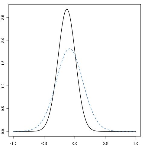
Following Ashley’s latest comments on Chapter 5 of Introducing Monte Carlo Methods with R, I realised Example 5.5 was totally off-the-mark! Not only the representation of the likelihood should have used prod instead of mean, not only the constant should call the val argument of integrate, not only integrate  uses lower and upper rather than from and to, but also the approximation is missing a scale factor of 10, squared root of the sample size… The corrected R code is thus

> cau=rcauchy(10^2)
> mcau=median(cau)
> rcau=diff(quantile(cau,c(.25,.75)))/sqrt(10^2)
> f=function(x){
+   z=dcauchy(outer(x,cau,FUN="-"))
+   apply(z,1,prod)}
> fcst=integrate(f,lower=-20,upper=20)$val
> ft=function(x){f(x)/fcst}
> g=function(x){dt((x-mcau)/rcau,df=49)/rcau}
> curve(ft,from=-1,to=1,xlab="",ylab="",lwd=2)
> curve(g,add=T,lty=2,col="steelblue",lwd=2)

and the corrected Figure 5.5 is therefore as follows. Note that the fit by the t distribution is not as perfect as before. A normal approximation would do better.

This mistake is most embarrassing and I cannot fathom how I came with this unoperating program! (The more embarrassing as Cauchy‘s house is about 1k away from mine…) I am thus quite grateful to Ashley for her detailed study of this example.

nlm [unused argument(s) (iter = 1)]

Posted in Books, R, Statistics with tags , , , , , on December 29, 2010 by xi'an

Ashley put the following comment on Chapter 5 of Introducing Monte Carlo Methods with R”:

I am reading chapter 5. I try to reproduced the result on page 128. The R codes don’t work on my laptop. When I try to run the following codes on page 128

> for (i in 1:(nlm(like,sta)$it)){
+ mmu=rbind(mmu,nlm(like,sta,iter=i)$est)}

I always get the error message

Error in f(x, …) : unused argument(s) (iter = 1)

It seems that the nlm function doesn’t accept the argument iter. I don’t know how to deal with it. I am in US. I guess the nlm version available to US R users is different from the version in EU. Please help.

And indeed with the most recent versions of R, like 2.12.1 on my own machine, calling nlm

> args(nlm)
function (f, p, ..., hessian = FALSE, typsize = rep(1, length(p)),
 fscale = 1, print.level = 0, ndigit = 12, gradtol = 1e-06,
 stepmax = max(1000 * sqrt(sum((p/typsize)^2)), 1000), steptol = 1e-06,
 iterlim = 100, check.analyticals = TRUE)

with the abbreviated argument iter instead of iterlim produces the above error message. This means the full syntax iterlim=i should now be used. In addition, the function nlm produces the minimum of the first argument f and like should thus be defined as

> like=function(mu){
+   -sum(log((.25*dnorm(da-mu[1])+.75*dnorm(da-mu[2]))))}

to end up with local maxima as on Figure 5.2. (Note: I do not think there are US versus EU versions of R…)

Ashley also pointed out another mistake on that page, namely that we used

> da=rbind(rnorm(10^2),2.5+rnorm(3*10^2))

instead of

> da=c(rnorm(10^2),2.5+rnorm(3*10^2))

to create a sample. Since the two normal samples have different sizes, rbind induces a duplication of the smaller sample, not what we intended!

Méthodes de Monte-Carlo avec R

Posted in Books, Kids, R, Statistics, University life with tags , , , , , on December 3, 2010 by xi'an

The translation of the book Introducing Monte Carlo Methods with R is close to being completed. The copy-editing and page-setting are done, I have received the cover proposal and am happy with it, so it should now go to production and be ready by early January, (earlier than the tentative end of February indicated on amazon) maybe in time for my R class students to get it before the exam. Thanks to the efforts of Pierre-André Cornillon and Eric Matzner (from the Université de Haute-Bretagne in Rennes), the move from the Use R! series format to the Pratique R series format was done seamlessly and effortlessly for me. (Again, thanks to the traductors who did produce their translations in sometimes less than a month!) I am curious to see how much of a market there is for the French translation… The Japanese translation is scheduled for August 2011 at the very least, but I am obviously not involved at all in this translation!

Graphical comparison of MCMC performance [arXiv:1011.445]

Posted in Books, R, Statistics with tags , , , , , , on November 22, 2010 by xi'an


A new posting on arXiv by Madeleine Thompson on a graphical tool for assessing performance. She has developed a software called SamplerCompare, implemented in R and C. The graphical evaluation plots “log density evaluations per iteration times autocorrelation time against a tuning parameter in a grid of plots where rows represent distributions and columns represent methods”. The autocorrelation time is evaluated in the same way as coda, which is the central package used in the convergence assessment chapter of Introducing Monte Carlo Methods with R because of its array of partial (if imperfect) indicators. Note that there is an approximation factor in the evaluation of the autocorrelation time because the MCMC output is represented as an AR(p) series, with a possible divergence artifact in the corresponding confidence interval if the AR(p) process is found to be non-stationary. When the simulation method (corresponding to columns in the above graphs) allows for an optimal value of its (cyber-)parameters, the performances exhibit a clear parabolic pattern (right graph), but this is not always the case (left graph). Graphical tools are always to be preferred to tables (a point Andrew would not rebuke!), However I do not see the point in simultaneously graphing the performances of different MCMC algorithms for different targets. This “wasted” dimension could instead be used for increasing to at least three the number of cyber-parameters evaluated by the method.