Archive for Jeffreys priors

re-revisiting Jeffreys

Posted in Books, pictures, Statistics, Travel, University life with tags , , , , , , , on October 16, 2015 by xi'an

Amster12Analytic Posteriors for Pearson’s Correlation Coefficient was arXived yesterday by Alexander Ly , Maarten Marsman, and Eric-Jan Wagenmakers from Amsterdam, with whom I recently had two most enjoyable encounters (and dinners!). And whose paper on Jeffreys’ Theory of Probability I recently discussed in the Journal of Mathematical Psychology.

The paper re-analyses Bayesian inference on the Gaussian correlation coefficient, demonstrating that for standard reference priors the posterior moments are (surprisingly) available in closed form. Including priors suggested by Jeffreys (in a 1935 paper), Lindley, Bayarri (Susie’s first paper!), Berger, Bernardo, and Sun. They all are of the form

\pi(\theta)\propto(1+\rho^2)^\alpha(1-\rho^2)^\beta\sigma_1^\gamma\sigma_2^\delta

and the corresponding profile likelihood on ρ is in “closed” form (“closed” because it involves hypergeometric functions). And only depends on the sample correlation which is then marginally sufficient (although I do not like this notion!). The posterior moments associated with those priors can be expressed as series (of hypergeometric functions). While the paper is very technical, borrowing from the Bateman project and from Gradshteyn and Ryzhik, I like it if only because it reminds me of some early papers I wrote in the same vein, Abramowitz and Stegun being one of the very first books I bought (at a ridiculous price in the bookstore of Purdue University…).

Two comments about the paper: I see nowhere a condition for the posterior to be proper, although I assume it could be the n>1+γ−2α+δ constraint found in Corollary 2.1 (although I am surprised there is no condition on the coefficient β). The second thing is about the use of this analytic expression in simulations from the marginal posterior on ρ: Since the density is available, numerical integration is certainly more efficient than Monte Carlo integration [for quantities that are not already available in closed form]. Furthermore, in the general case when β is not zero, the cost of computing infinite series of hypergeometric and gamma functions maybe counterbalanced by a direct simulation of ρ and both variance parameters since the profile likelihood of this triplet is truly in closed form, see eqn (2.11). And I will not comment the fact that Fisher ends up being the most quoted author in the paper!

Moment conditions and Bayesian nonparametrics

Posted in R, Statistics, University life with tags , , , , , , , , , , on August 6, 2015 by xi'an

Luke Bornn, Neil Shephard, and Reza Solgi (all from Harvard) have arXived a pretty interesting paper on simulating targets on a zero measure set. Although it is not initially presented this way, but rather in non-parametric terms as moment conditions

\mathbb{E}_\theta[g(X,\beta)]=0

where θ is the parameter of the sampling distribution, constrained by the value of β. (Which also contains quantile regression.) The very problem of simulating under a hard constraint has been bugging me for years and it is hence very exciting to see them come up with a proposal towards solving this difficulty! Even though it is restricted here to observations with a finite support (hence allowing for the use of a parametric Dirichlet prior). One interesting extension (Section 3.6) processed in the paper is the case when the support is unknown, but finite, with some points in the support being unobserved. Maybe connecting with non-parametrics if a prior is added on the number of unobserved points.

The setting of constricting θ via a parameterised moment condition relates to moment defined econometrics models, in a similar spirit to Gallant’s paper I recently discussed, but equally to empirical likelihood, which would then benefit from a fully Bayesian treatment thanks to the approach advocated by the authors.

bornnshepardDespite the zero-measure difficulty, or more exactly the non-linear manifold structure of the parameter space, for instance

β = log {θ/(1-θ)}

the authors manage to define a “projected” [my words] measure on the set of admissible pairs (β,θ). In a sense this is related with the choice of a certain metric, but the so-called Hausdorff reference measure allows for an automated definition of the original prior. It took me a (wee) while to spot (p.7) that the starting point was not a (unconstrained) prior on that (unconstrained) pair (β,θ) but directly on the manifold

\mathbb{E}_\theta[g(X,\beta)]=0.

Which makes its construction a difficulty. Even though, as noted in Section 4, all that we need is a prior over θ since the Hausdorff-Jacobian identity defines the “joint”, in a sort of backward way. (This is a wee bit confusing in that β being a transform of θ, all we need is a prior over θ, but we nonetheless end up with a different density on the joint distribution on the pair (β,θ). Any connection with incompatible priors merged together into a consensus prior?) Another question extending the scope of the paper would be to define Jeffreys’ or reference priors in this manifold sense.

The authors also discuss (Section 4.3) the problem I originally thought they were processing, namely starting from an unconstrained pair (β,θ) and it corresponding prior. The projected prior can then be defined based on a version of the original density on the constrained space, but it is definitely arbitrary. In that sense the paper does not address the general problem.

bornnshepard1“…traditional simulation algorithms will fail because the prior and the posterior of the model are supported on a zero Lebesgue measure set…” (p.10)

I somewhat resist this presentation through the measure zero set: once the prior is defined on a manifold, the fact that it is a measure zero set in a larger space is moot. Provided one can simulate a proposal over that manifold, e.g., a random walk, absolutely continuous wrt the same dominating measure, and compute or estimate a Metropolis-Hastings ratio of densities against a common measure, one can formally run MCMC on manifolds as well as regular Euclidean spaces. A first and theoretically straightforward (?) solution is to solve the constraint

\mathbb{E}_\theta[g(X,\beta)]=0

in β=β(θ). Then the joint prior p(β,θ) can be projected by the Hausdorff projection into p(θ). For instance, in the case of the above logit transform, the projected density is

p(θ)=p(β,θ) {1+1/θ²(1-θ)²}½

In practice, the inversion may be too costly and Bornn et al. directly simulate the pair (β,θ) within the manifold capitalising on the fact that the constraint is linear in θ given β. Indeed, in this setting, β is unconstrained and θ can be simulated from a proposal restricted to the hyperplane. Gibbs-like.

Is Jeffreys’ prior unique?

Posted in Books, Statistics, University life with tags , , , , , on March 3, 2015 by xi'an

“A striking characterisation showing the central importance of Fisher’s information in a differential framework is due to Cencov (1972), who shows that it is the only invariant Riemannian metric under symmetry conditions.” N. Polson, PhD Thesis, University of Nottingham, 1988

Following a discussion on Cross Validated, I wonder whether or not the affirmation that Jeffreys’ prior was the only prior construction rule that remains invariant under arbitrary (if smooth enough) reparameterisation. In the discussion, Paulo Marques mentioned Nikolaj Nikolaevič Čencov’s book, Statistical Decision Rules and Optimal Inference, Russian book from 1972, of which I had not heard previously and which seems too theoretical [from Paulo’s comments] to explain why this rule would be the sole one. As I kept looking for Čencov’s references on the Web, I found Nick Polson’s thesis and the above quote. So maybe Nick could tell us more!

However, my uncertainty about the uniqueness of Jeffreys’ rule stems from the fact that, f I decide on a favourite or reference parametrisation—as Jeffreys indirectly does when selecting the parametrisation associated with a constant Fisher information—and on a prior derivation from the sampling distribution for this parametrisation, I have derived a parametrisation invariant principle. Possibly silly and uninteresting from a Bayesian viewpoint but nonetheless invariant.

delayed acceptance with prefetching

Posted in Books, Kids, Statistics, Travel, University life with tags , , , , , , , on June 12, 2014 by xi'an

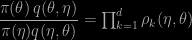
In a somewhat desperate rush (started upon my return from Iceland and terminated on my return from Edinburgh), Marco Banterle, Clara Grazian and I managed to complete and submit our paper by last Friday evening… It is now arXived as well. The full title of the paper is Accelerating Metropolis-Hastings algorithms: Delayed acceptance with prefetching and the idea behind the generic acceleration is (a) to divide the acceptance step into parts, towards a major reduction in computing time that outranks the corresponding reduction in acceptance probability and (b) to exploit this division to build a dynamic prefetching algorithm. The division is to break the prior x likelihood target into a product such that some terms are much cheaper than others. Or equivalently to represent the acceptance-rejection ratio in the Metropolis-Hastings algorithm as

\dfrac{\pi(\theta)\,q(\theta,\eta)}{\pi(\eta)q(\eta,\theta)} = \prod_{k=1}^d \rho_k(\eta,\theta)

again with significant differences in the computing cost of those terms. Indeed, this division can be exploited by checking for each term sequentially, in the sense that the overall acceptance probability

\prod_{k=1}^d \min\left\{\rho_k(\eta,\theta),1\right\}

is associated with the right (posterior) target! This lemma can be directly checked via the detailed balance condition, but it is also a consequence of a 2005 paper by Andrès Christen and Colin Fox on using approximate transition densities (with the same idea of gaining time: in case of an early rejection, the exact target needs not be computed). While the purpose of the recent [commented] paper by Doucet et al. is fundamentally orthogonal to ours, a special case of this decomposition of the acceptance step in the Metropolis–Hastings algorithm can be found therein. The division of the likelihood into parts also allows for a precomputation of the target solely based on a subsample, hence gaining time and allowing for a natural prefetching version, following recent developments in this direction. (Discussed on the ‘Og.) We study the novel method within two realistic environments, the fi rst one made of logistic regression targets using benchmarks found in the earlier prefetching literature and a second one handling an original analysis of a parametric mixture model via genuine Jeffreys priors. [As I made preliminary notes along those weeks using the ‘Og as a notebook, several posts on the coming days will elaborate on the above.]

noninformative priors for mixtures

Posted in Books, Statistics, University life with tags , , , , , , , , on May 26, 2014 by xi'an

“A novel formulation of the mixture model is introduced, which includes the prior constraint that each Gaussian component is always assigned a minimal number of data points. This enables noninformative improper priors such as the Jeffreys prior to be placed on the component parameters. We demonstrate difficulties involved in specifying a prior for the standard Gaussian mixture model, and show how the new model can be used to overcome these. MCMC methods are given for efficient sampling from the posterior of this model.” C. Stoneking

cover of Mixture Estimation and ApplicationsFollowing in the theme of the Jeffreys’ post of two weeks ago, I spotted today a newly arXived paper about using improper priors for mixtures…and surviving it! It is entitled “Bayesian inference of Gaussian mixture models with noninformative priors” and written by Colin Stoneking at ETH Zürich. As mentioned in the previous post, one specificity of our 1990-1994 paper on mixture with Jean Diebolt was to allow for improper priors by imposing at least two observations per component. The above abstract thus puzzled me until I found on page 3 that the paper was indeed related to ours (and Larry’s 2000 validation)! Actually, I should not complain about citations of my earlier works on mixtures as they cover seven different papers, but the bibliography is somewhat missing the paper we wrote with George Casella and Marty Wells in Statistical Methodology in 2004 (this was actually the very first paper of this new journal!), where we show that conjugate priors allow for the integration of the weights, resulting in a close-form expression for the distribution of the partition vector. (This was also extended in the chapter “Exact Bayesian Analysis of Mixtures” I wrote with Kerrie Mengersen in our book Mixtures: Estimation and Applications.)

“There is no well-founded, general method to choose the parameters of a given prior to make it weakly informative for Gaussian mixtures.” C. Stoneking

The first part of the paper shows why looking for weakly informative priors is doomed to fail in this mixture setting: there is no stabilisation as hyperparameters get towards the border (between proper-ness and improper-ness), and on the opposite the frequency of appearances of empty components grows steadily to 100%…  The second part gets to the reassessment of our 1990 exclusion trick, first considering that it is not producing a true posterior, then criticising Larry’s 2000 analysis as building a data-dependent “prior”, and at last proposing a reformulation where the exclusion of the empty components and those with one allocated observation becomes part of the “prior” (albeit a prior on the allocation vector). In fine, the posterior thus constructed remains the same as ours, with a message that if we start our model as the likelihood of the sample excluding empty or single-observation terms, we can produce a proper Bayesian analysis. (Except for a missing if minor renormalisation.) This leads me to wonder about the conclusion that inference about the (unknown) number of components in the mixture being impossible from this perspective. For instance, we could define fractional Bayes factors à la O’Hagan (1995) this way, i.e. starting from the restricted likelihood and taking a fraction of the likelihood to make the posterior proper, then using the remaining fraction to compute a Bayes factor. (Fractional Bayes factors do not work for the regular likelihood of a Gaussian mixture, irrespective of the sample size.)