Archive for marginalisation paradoxes

the Flatland paradox

Posted in Books, Kids, R, Statistics, University life with tags , , , , , , , , on May 13, 2015 by xi'an

Pierre Druilhet arXived a note a few days ago about the Flatland paradox (due to Stone, 1976) and his arguments against the flat prior. The paradox in this highly artificial setting is as follows:  Consider a sequence θ of N independent draws from {a,b,1/a,1/b} such that

  1. N and θ are unknown;
  2. a draw followed by its inverse and this inverse are removed from θ;
  3. the successor x of θ is observed, meaning an extra draw is made and the above rule applied.

Then the frequentist probability that x is longer than θ given θ is at least 3/4—at least because θ could be zero—while the posterior probability that x is longer than θ given x is 1/4 under the flat prior over θ. Paradox that 3/4 and 1/4 clash. Not so much of a paradox because there is no joint probability distribution over (x,θ).

The paradox was actually discussed at length in Larry Wasserman’s now defunct Normal Variate. From which I borrowed Larry’s graphical representation of the four possible values of θ given the (green) endpoint of x. Larry uses the Flatland paradox hammer to fix another nail on the coffin he contemplates for improper priors. And all things Bayes. Pierre (like others before him) argues against the flat prior on θ and shows that a flat prior on the length of θ leads to recover 3/4 as the posterior probability that x is longer than θ.

As I was reading the paper in the métro yesterday morning, I became less and less satisfied with the whole analysis of the problem in that I could not perceive θ as a parameter of the model. While this may sound a pedantic distinction, θ is a latent variable (or a random effect) associated with x in a model where the only unknown parameter is N, the total number of draws used to produce θ and x. The distributions of both θ and x are entirely determined by N. (In that sense, the flatland paradox can be seen as a marginalisation paradox in that an improper prior on N cannot be interpreted as projecting a prior on θ.) Given N, the distribution of x of length l(x) is then 1/4N times the number of ways of picking (N-l(x)) annihilation steps among N. Using a prior on N like 1/N , which is improper, then leads to favour the shortest path as well. (After discussing the issue with Pierre Druilhet, I realised he had a similar perspective on the issue. Except that he puts a flat prior on the length l(x).) Looking a wee bit further for references, I also found that Bruce Hill had adopted the same perspective of a prior on N.
Approximate Integrated Likelihood via ABC methods

Posted in Books, Statistics, University life with tags , , , , , , , , on March 13, 2014 by xi'an

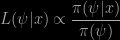
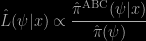
My PhD student Clara Grazian just arXived this joint work with Brunero Liseo on using ABC for marginal density estimation. The idea in this paper is to produce an integrated likelihood approximation in intractable problems via the ratio

L(\psi|x)\propto \dfrac{\pi(\psi|x)}{\pi(\psi)}

both terms in the ratio being estimated from simulations,

\hat L(\psi|x) \propto \dfrac{\hat\pi^\text{ABC}(\psi|x)}{\hat\pi(\psi)}

(with possible closed form for the denominator). Although most of the examples processed in the paper (Poisson means ratio, Neyman-Scott’s problem, g-&-k quantile distribution, semi-parametric regression) rely on summary statistics, hence de facto replacing the numerator above with a pseudo-posterior conditional on those summaries, the approximation remains accurate (for those examples). In the g-&-k quantile example, Clara and Brunero compare our ABC-MCMC algorithm with the one of Allingham et al. (2009, Statistics & Computing): the later does better by not replicating values in the Markov chain but instead proposing a new value until it is accepted by the usual Metropolis step. (Although I did not spend much time on this issue, I cannot see how both approaches could be simultaneously correct. Even though the outcomes do not look very different.) As noted by the authors, “the main drawback of the present approach is that it requires the use of proper priors”, unless the marginalisation of the prior can be done analytically. (This is an interesting computational problem: how to provide an efficient approximation to a marginal density of a σ-finite measure, assuming this density exists.)

Clara will give a talk at CREST-ENSAE today about this work, in the Bayes in Paris seminar: 2pm in room 18.

Robins and Wasserman

Posted in Statistics, Travel, University life with tags , , , , on January 17, 2013 by xi'an

entrance to Banaras Hindu University, with the huge ISBA poster, Varanasi, Jan. 10, 2013As I attended Jamie Robins’ session in Varanasi and did not have a clear enough idea of the Robbins and Wasserman paradox to discuss it viva vocce, here are my thoughts after reading Larry’s summary. My first reaction was to question whether or not this was a Bayesian statistical problem (meaning why should I be concered with the problem). Just as the normalising constant problem was not a statistical problem. We are estimating an integral given some censored realisations of a binomial depending on a covariate through an unknown function θ(x). There is not much of a parameter. However, the way Jamie presented it thru clinical trials made the problem sound definitely statistical. So end of the silly objection. My second step is to consider the very point of estimating the entire function (or infinite dimensional parameter) θ(x) when only the integral ψ is of interest. This is presumably the reason why the Bayesian approach fails as it sounds difficult to consistently estimate θ(x) under censored binomial observations, while ψ can be. Of course, if we want to estimate the probability of a success like ψ going through functional estimation this sounds like overshooting. But the Bayesian modelling of the problem appears to require considering all unknowns at once, including the function θ(x) and cannot forget about it. We encountered a somewhat similar problem with Jean-Michel Marin when working on the k-nearest neighbour classification problem. Considering all the points in the testing sample altogether as unknowns would dwarf the training sample and its information content to produce very poor inference. And so we ended up dealing with one point at a time after harsh and intense discussions! Now, back to the Robins and Wasserman paradox, I see no problem in acknowledging a classical Bayesian approach cannot produce a convergent estimate of the integral ψ. Simply because the classical Bayesian approach is an holistic system that cannot remove information to process a subset of the original problem. Call it the curse of marginalisation. Now, on a practical basis, would there be ways of running simulations of the missing Y’s when π(x) is known in order to achieve estimates of ψ? Presumably, but they would end up with a frequentist validation…

Confidence distributions

Posted in Books, Statistics, Travel, University life with tags , , , , , , , , on June 11, 2012 by xi'an

I was asked by the International Statistical Review editor, Marc Hallin, for a discussion of the paper “Confidence distribution, the frequentist distribution estimator of a parameter — a review” by Min-ge Xie and Kesar Singh, both from Rutgers University. Although the paper is not available on-line, similar and recent reviews and articles can be found, in an 2007 IMS Monograph and a 2012 JASA paper both with Bill Strawderman, as well as a chapter in the recent Fetschrift for Bill Strawderman. The notion of confidence distribution is quite similar to the one of fiducial distribution, introduced by R.A. Fisher, and they both share in my opinion the same drawback, namely that they aim at a distribution over the parameter space without specifying (at least explicitly) a prior distribution. Furthermore, the way the confidence distribution is defined perpetuates the on-going confusion between confidence and credible intervals, in that the cdf on the parameter θ is derived via the inversion of a confidence upper bound (or, equivalently, of a p-value…) Even though this inversion properly defines a cdf on the parameter space, there is no particular validity in the derivation. Either the confidence distribution corresponds to a genuine posterior distribution, in which case I think the only possible interpretation is a Bayesian one. Or  the confidence distribution does not correspond to a genuine posterior distribution, because no prior can lead to this distribution, in which case there is a probabilistic impossibility in using this distribution.  Thus, as a result, my discussion (now posted on arXiv) is rather negative about the benefits of this notion of confidence distribution.

One entry in the review, albeit peripheral, attracted my attention. The authors mention a tech’ report where they exhibit a paradoxical behaviour of a Bayesian procedure: given a (skewed) prior on a pair (p0,p1), and a binomial likelihood, the posterior distribution on p1-p0 has its main mass in the tails of both the prior and the likelihood (“the marginal posterior of d = p1-p0 is more extreme than its prior and data evidence!”). The information provided in the paper is rather sparse on the genuine experiment and looking at two possible priors exhibited nothing of the kind… I went to the authors’ webpages and found a more precise explanation on Min-ge Xie’s page:

Although the contour plot of the posterior distribution sits between those of the prior distribution and the likelihood function, its projected peak is more extreme than the other two. Further examination suggests that this phenomenon is genuine in binomial clinical trials and it would not go away even if we adopt other (skewed) priors (for example, the independent beta priors used in Joseph et al. (1997)). In fact, as long as the center of a posterior distribution is not on the line joining the two centers of the joint prior and likelihood function (as it is often the case with skewed distributions), there exists a direction along which the marginal posterior fails to fall between the prior and likelihood function of the same parameter.

and a link to another paper. Reading through the paper (and in particular Section 4), it appears that the above “paradoxical” picture is the result of the projections of the joint distributions represented in this second picture. By projection, I presume the authors mean integrating out the second component, e.g. p1+p0. This indeed provides the marginal prior of p1-p0, the marginal posterior of p1-p0, but…not the marginal likelihood of p1-p0! This entity is not defined, once again because there is no reference measure on the parameter space which could justify integrating out some parameters in the likelihood. (Overall, I do not think the “paradox” is overwhelming: the joint posterior distribution does precisely the merging of prior and data information we would expect and it is not like the marginal posterior is located in zones with zero prior probability and zero (profile) likelihood. I am also always wary of arguments based on modes, since those are highly dependent on parameterisation.)

Most unfortunately, when searching for more information on the authors’ webpages, I came upon the sad news that Professor Singh had passed away three weeks ago, at the age of 56.  (Professor Xie wrote a touching eulogy of his friend and co-author.) I had only met briefly with Professor Singh during my visit to Rutgers two months ago, but he sounded like an academic who would have enjoyed the kind of debate drafted by my discussion. To the much more important loss to family, friends and faculty represented by Professor Singh demise, I thus add the loss of missing the intellectual challenge of crossing arguments with him. And I look forward discussing the issues with the first author of the paper, Professor Xie.

improper priors, incorporated

Posted in Books, Statistics, University life with tags , , , , , , , , on January 11, 2012 by xi'an

“If a statistical procedure is to be judged by a criterion such as a conventional loss function (…) we should not expect optimal results from a probabilistic theory that demands multiple observations and multiple parameters.” P. McCullagh & H. Han

Peter McCullagh and Han Han have just published in the Annals of Statistics a paper on Bayes’ theorem for improper mixtures. This is a fascinating piece of work, even though some parts do elude me… The authors indeed propose a framework based on Kingman’s Poisson point processes that allow to include (countable) improper priors in a coherent probabilistic framework. This framework requires the definition of a test set A in the sampling space, the observations being then the events Y∩ A, Y being an infinite random set when the prior is infinite. It is therefore complicated to perceive this representation in a genuine Bayesian framework, i.e. for a single observation, corresponding to a single parameter value. In that sense it seems closer to the original empirical Bayes, à la Robbins.

“An improper mixture is designed for a generic class of problems, not necessarily related to one another scientifically, but all having the same mathematical structure.” P. McCullagh & H. Han

The paper thus misses in my opinion a clear link with the design of improper priors. And it does not offer a resolution of the  improper prior Bayes factor conundrum. However, it provides a perfectly valid environment for working with improper priors. For instance, the final section on the marginalisation “paradoxes” is illuminating in this respect as it does not demand  using a limit of proper priors.