Archive for normal distribution

uniform correlation mixtures

Posted in Books, pictures, Statistics, University life with tags , , , , , , , , , on December 4, 2015 by xi'an

Philadelphia, Nov. 01, 2010Kai Zhang and my friends from Wharton, Larry Brown, Ed George and Linda Zhao arXived last week a neat mathematical foray into the properties of a marginal bivariate Gaussian density once the correlation ρ is integrated out. While the univariate marginals remain Gaussian (unsurprising, since these marginals do not depend on ρ in the first place), the joint density has the surprising property of being

[1-Φ(max{|x|,|y|})]/2

which turns an infinitely regular density into a density that is not even differentiable everywhere. And which is constant on squares rather than circles or ellipses. This is somewhat paradoxical in that the intuition (at least my intuition!) is that integration increases regularity… I also like the characterisation of the distributions factorising through the infinite norm as scale mixtures of the infinite norm equivalent of normal distributions. The paper proposes several threads for some extensions of this most surprising result. Other come to mind:

  1. What happens when the Jeffreys prior is used in place of the uniform? Or Haldane‘s prior?
  2. Given the mixture representation of t distributions, is there an equivalent for t distributions?
  3. Is there any connection with the equally surprising resolution of the Drton conjecture by Natesh Pillai and Xiao-Li Meng?
  4. In the Khintchine representation, correlated normal variates are created by multiplying a single χ²(3) variate by a vector of uniforms on (-1,1). What are the resulting variates for other degrees of freedomk in the χ²(k) variate?
  5. I also wonder at a connection between this Khintchine representation and the Box-Müller algorithm, as in this earlier X validated question that I turned into an exam problem.

a programming bug with weird consequences

Posted in Kids, pictures, R, Statistics, University life with tags , , , , , , on November 25, 2015 by xi'an

One student of mine coded by mistake an independent Metropolis-Hastings algorithm with too small a variance in the proposal when compared with the target variance. Here is the R code of this implementation:

[sourcecode language=”r” gutter=”false”]
#target is N(0,1)
#proposal is N(0,.01)
T=1e5
prop=x=rnorm(T,sd=.01)
ratop=dnorm(prop,log=TRUE)-dnorm(prop,sd=.01,log=TRUE)
ratav=ratop[1]
logu=ratop-log(runif(T))
for (t in 2:T){
if (logu[t]>ratav){
x[t]=prop[t];ratav=ratop[t]}else{x[t]=x[t-1]}
}
[/sourcecode]

It produces outputs of the following shape
smalvarwhich is quite amazing because of the small variance. The reason for the lengthy freezes of the chain is the occurrence with positive probability of realisations from the proposal with very small proposal density values, as they induce very small Metropolis-Hastings acceptance probabilities and are almost “impossible” to leave. This is due to the lack of control of the target, which is flat over the domain of the proposal for all practical purposes. Obviously, in such a setting, the outcome is unrelated with the N(0,1) target!

It is also unrelated with the normal proposal in that switching to a t distribution with 3 degrees of freedom produces a similar outcome:

It is only when using a Cauchy proposal that the pattern vanishes:

simulation by inverse cdf

Posted in Books, Kids, R, Statistics, University life with tags , , , , , on January 14, 2015 by xi'an

Another Cross Validated forum question that led me to an interesting (?) reconsideration of certitudes! When simulating from a normal distribution, is Box-Muller algorithm better or worse than using the inverse cdf transform? My first reaction was to state that Box-Muller was exact while the inverse cdf relied on the coding of the inverse cdf, like qnorm() in R. Upon reflection and commenting by other members of the forum, like William Huber, I came to moderate this perspective since Box-Muller also relies on transcendental functions like sin and log, hence writing

X=\sqrt{-2\log(U_1)}\,\sin(2\pi U_2)

also involves approximating in the coding of those functions. While it is feasible to avoid the call to trigonometric functions (see, e.g., Algorithm A.8 in our book), the call to the logarithm seems inescapable. So it ends up with the issue of which of the two functions is better coded, both in terms of speed and precision. Surprisingly, when coding in R, the inverse cdf may be the winner: here is the comparison I ran at the time I wrote my comments

[sourcecode language=”r” gutter=”false”]
> system.time(qnorm(runif(10^8)))
sutilisateur système écoulé
10.137 0.120 10.251
> system.time(rnorm(10^8))
utilisateur système écoulé
13.417 0.060 13.472`
[/sourcecode]

However re-rerunning it today, I get opposite results (pardon my French, I failed to turn the messages to English):

[sourcecode language=”r” gutter=”false”]
> system.time(qnorm(runif(10^8)))
utilisateur système écoulé
10.137 0.144 10.274
> system.time(rnorm(10^8))
utilisateur système écoulé
7.894 0.060 7.948
[/sourcecode]

(There is coherence in the system time, which shows rnorm as twice as fast as the call to qnorm.) In terms, of precision, I could not spot a divergence from normality, either through a ks.test over 10⁸ simulations or in checking the tails:

“Only the inversion method is inadmissible because it is slower and less space efficient than all of the other methods, the table methods excepted”. Luc Devroye, Non-uniform random variate generation, 1985

Update: As pointed out by Radford Neal in his comment, the above comparison is meaningless because the function rnorm() is by default based on the inversion of qnorm()! As indicated by Alexander Blocker in another comment, to use an other generator requires calling RNG as in

[sourcecode language=”r” gutter=”false”]
RNGkind(normal.kind = “Box-Muller”)
[/sourcecode]

(And thanks to Jean-Louis Foulley for salvaging this quote from Luc Devroye, which does not appear to apply to the current coding of the Gaussian inverse cdf.)

Forsythe’s algorithm

Posted in R, Statistics with tags , , , , , , on May 9, 2010 by xi'an

In connection with the Bernoulli factory post of last week, Richard Brent arXived a short historical note recalling George Forsythe’s algorithm for simulating variables with density \exp\{-G(x)\} when 0\le G(x)\le 1 (the extension to any upper bound is straightforward). The idea is to avoid computing the exponential function by simulating uniforms u_i until

G(x) \ge u_1 \ldots \ge u_{n-1} \le u_n

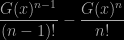
since the probability of this event is

\dfrac{G(x)^{n-1}}{(n-1)!} - \dfrac{G(x)^{n}}{n!}

its expectation is \exp\{G(x)\} and the probability that n is even is \exp\{-G(x)\}. This turns into a generation method if the support of G is bounded. In relation with the Bernoulli factory problem, I think this has potential applications in that, when the function G(x) is replaced with an unbiased estimator the subsequent steps remain valid. This approach would indeed involve computing one single value of G(x), but this is also the case with Latuszyński et al.’s and our solutions… So I am uncertain as to whether or not this has practical implications. (Brent mentions normal simulation but this is more history than methodology.)