Archive for Python

probably overthinking it [book review]

Posted in Books, Statistics, University life with tags , , , , , , , , , , , , , , , , , , , , on December 13, 2023 by xi'an

Probably overthinking it, written by Allen B. Downey (who wrote a series of books starting with Think, like Think Python, Think Bayes, Think Stats), belongs to this numerous collection of introductory books that aim at making statistics more palatable and enticing to the general public by making the fundamental concepts more intuitive and building upon real life examples. I would thus stop short of calling it “essential guide” as in the first flap of the dust jacket, since there exist many published books with a similar goal, some of which were actually reviews here. Now, there are ideas and examples therein I could borrow for my introductory stats course, except that I will cease teaching it next year! For instance, there are lots of examples related to COVID, which is great to engage (enrage?) the readers.

The book is quite pleasant to read, does not shy from mathematical formulae, and covers notions such as probability distributions, the Simpson, the Preston, the inspection, the Berkson paradoxes, and even some words on causality, sometimes at excessive lengths. (I have always been an adept of the concise church when it comes to textbook examples and fear that the multiplication of illustrations of a given concept may prove counterproductive.) The early chapters are heavily focussed on the Gaussian (or Normal) distribution. Making it appear as essential for conducting statistical analysis. When it does not, as in the ELO example, the explanations of a correction are less convincing.

I appreciated the book approach to model fit via the comparison of empirical cdfs with hypothetical ones. Also of primary interest is the systematic recourse to simulation, aka generative models, albeit without a systematic proper description. In the chapter (Chap 5) about durations, I think there are missed opportunities like the distributions of extremes (p 82) or the forgetfulness property of the Exponential distribution. Instead the focus is slightly diverging towards non-statistical issues on demography by the end of the chapter, with a potential for confusion between the Gomperz law and the Gomperz distribution. The Berkson paradox (Chap 6) is well-explained in terms of non-random populations (and reminded me when, years ago, when we tried to predict the first year success probability of undergrad applicants from their high school maths grade, the regression coefficient estimate ended up negative). Distributions of extremes do appear in Chap 8, if again seeking an ideal generic distribution seems to me rather misguided and misguiding. I would also argue that the author is missing the point of Taleb’s black swans by arguing in favour of a better modelling, when the later argues against the very predictability of extreme events in a non-stationary financial world… The chapter on fairness and fallacy (Chap 9) is actually about false positive/negative rates in different populations hence the ensuing unfairness (or the base fallacy). In that chapter there is no mention of Bayes (reserved for Think Bayes?!), but it is hitting hard enough at anti-vaxers (who will most likely not read the book). And does it again in the Simpson paradox chapter (Chap 10), whose proliferation is further stressed the following chapter on people becoming less racist or sexist or homophobic when they age, despite the proportion of racist/sexist/homophobic responses to a specific survey (GSS/Pew) increasing with age. This is prolonged into the rather minor final chapter.

Now that I have read the book, during a balmy afternoon in St Kilda (after an early start in the train to De Gaulle airport in freezing temperatures), I am a bit uncertain at what to make of it in terms of impact on the general public. For sure, the stories that accumulate chapter after chapter are nice and well argued, while introducing useful statistical concepts, but I do not see readers equipped enough to handle daily statistics with more than an healthy dose of scepticism, which obviously is a first step in the right direction!

Some nitpicking : the book is missing the historical connection to Quetelet’s “average man” when referring to the notion. And a potential explanation for the (approximate) log-Gaussianity of weights of individuals in a population through the fact that it is a volume, hence a third power of a sort.  Although birth weights are roughly Normal which kill my argument. I remain puzzled by the title, possibly missing a cultural reference (as there are tee-shirts sold with this sentence). It is the same as the name of a blog run by the author since 2011 and a fodder for the book. And the cover is terrible, breaking the words to fit the width making no sense, if I am not overthinking it! As often the book is rather US centric, although making no mention of US having much higher infant death rates than countries with similar GDPs when this data is discussed.

[Disclaimer about potential self-plagiarism: this post or an edited version will eventually appear in my Books Review section in CHANCE.]

grasshoppers for pythons

Posted in Books, Kids, pictures, R, Statistics with tags , , , , , , on May 18, 2023 by xi'an

Following my earlier post on the terrible performances of ChatGPT for a grasshopping riddle, Bob Carpenter sent me his interaction with GPT4, using the same entry. Here is the python code outcome he obtained. The code is running  and the answer is correct.

BC: Thanks. Can you write a python program to simulate the final position of the grasshopper to within machine tolerance using single-precision floating point arithmetic?

GPT4: Sure, here’s a simple Python program that simulates the grasshopper’s journey using single-precision floating point arithmetic, specifically the float32 data type from the numpy library. It continues until the jump size is less than the machine epsilon for float32, which is the smallest representable positive number such that 1.0 + eps != 1.0.

import numpy as np
import random

# Initialize position and jump size
position = np.float32(0.0)
jump = np.float32(0.5)

# Get machine epsilon for float32
eps = np.finfo(np.float32).eps

# Perform jumps until jump size is less than machine epsilon
while jump > eps:
# Choose direction randomly
direction = random.choice([-1, 1])
# Update position
position += direction * jump
# Halve the jump size
jump /= 2

Remember that this program only simulates a single instance of the grasshopper’s journey. If you ran it multiple times, you would get different results each time due to the randomness in the choice of direction. However, on average, you should expect the final positions to be around 0, as per our mathematical analysis earlier. The absolute distance from the origin, however, will vary and, on average, should be close to 1/2.
print(“Final position:”, position)

BC: can you write a program to calculate the expected length of the final position from the origin?

import numpy as np
import random

# Define the number of simulations
num_simulations = 100000

# Initialize an array to store the final positions
final_positions = np.zeros(num_simulations, dtype=np.float32)

# Perform each simulation
for i in range(num_simulations):
# Initialize position and jump size
position = np.float32(0.0)
jump = np.float32(0.5)

# Get machine epsilon for float32
eps = np.finfo(np.float32).eps

# Perform jumps until jump size is less than machine epsilon
while jump > eps:
# Choose direction randomly
direction = random.choice([-1, 1])
# Update position
position += direction * jump
# Halve the jump size
jump /= 2

# Store the final position
final_positions[i] = position

# Calculate the expected length of the final position from the origin
expected_length = np.mean(np.abs(final_positions))

print(“Expected length of the final position from the origin:”, expected_length)

The Effect [book review]

Posted in Books, R, Running, Statistics, University life with tags , , , , , , , , , , , , , , , , , , , , , on March 10, 2023 by xi'an

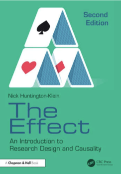
While it sounds like the title of a science-fiction catastrophe novel or of a (of course) convoluted nouveau roman, this book by Nick Huntington-Klein is a massive initiation to econometrics and causality. As explained by the subtitle, An Introduction to Research Design and Causality.

This is a hüûüge book, actually made of two parts that could have been books (volumes?). And covering three langages, R, Stata, and Python, which should have led to three independent books. (Seriously, why print three versions when you need at best one?!)  I carried it with me during my vacations in Central Québec, but managed to loose my notes on the first part, which means missing the opportunity for biased quotes! It was mostly written during the COVID lockdown(s), which may explain for a certain amount of verbosity and rambling around.

“My mom loved the first part of the book and she is allergic to statistics.”

The first half (which is in fact a third!) is conceptual (and chatty) and almost formula free, based on the postulate that “it’s a pretty slim portion of students who understand a method because of an equation” (p.xxii). For this reader (or rather reviewer) and on explanations through example, it makes the reading much harder as spotting the main point gets harder (and requires reading most sentences!). And a very slow start since notations and mathematical notions have to be introduced with an excess of caution (as in the distinction between Latin and Greek symbols, p.36). Moving through single variable models, conditional distributions, with a lengthy explanation of how OLS are derived, data generating process and identification (of causes), causal diagrams, back and front doors (a recurrent notion within the book),  treatment effects and a conclusion chapter.

“Unlike statistical research, which is completely made of things that are at least slightly false, statistics itself is almost entirely true.” (p.327)

The second part, called the Toolbox, is closer to a classical introduction to econometrics, albeit with a shortage of mathematics (and no proof whatsoever), although [warning!] logarithms, polynomials, partial derivatives and matrices are used. Along with a consequent (3x) chunk allocated to printed codes, the density of the footnotes significantly increases in this section. It covers an extensive chapter on regression (including testing practice, non-linear and generalised linear models, as well as basic bootstrap without much warning about its use in… regression settings, and LASSO),  one on matching (with propensity scores, kernel weighting, Mahalanobis weighting, one on  simulation, yes simulation! in the sense of producing pseudo-data from known generating processes to check methods, as well as bootstrap (with resampling residuals making at last an appearance!), fixed and random effects (where the author “feels the presence of Andrew Gelman reaching through time and space to disagree”, p.405). The chapter on event studies is about time dependent data with a bit of ARIMA prediction (but nothing on non-stationary series and unit root issues). The more exotic chapters cover (18) difference-in-differences models (control vs treated groups, with John Snow pumping his way in), (19) instrumental variables (aka the minor bane of my 1980’s econometrics courses), with double least squares and generalised methods of moments (if not the simulated version), (20) discontinuity (i.e., changepoints), with the limitation of having a single variate explaining the change, rather than an unknown combination of them, and a rather pedestrian approach to the issue, (iv) other methods (including the first mention of machine learning regression/prediction and some causal forests), concluding with an “Under the rug” portmanteau.

Nothing (afaict) on multivariate regressed variates and simultaneous equations. Hardly an occurrence of Bayesian modelling (p.581), vague enough to remind me of my first course of statistics and the one-line annihilation of the notion.

Duh cover, but nice edition, except for the huge margins that could have been cut to reduce the 622 pages by a third (and harnessed the tendency of the author towards excessive footnotes!). And an unintentional white line on p.238! Cute and vaguely connected little drawings at the head of every chapter (like the head above). A rather terse matter index (except for the entry “The first reader to spot this wins ten bucks“!), which should have been completed with an acronym index.

“Calculus-heads will recognize all of this as taking integrals of the density curve. Did you know there’s calculus hidden inside statistics? The things your professor won’t tell you until it’s too late to drop the class.

Obviously I am biased in that I cannot negatively comment on an author running 5:37 a mile as, by now, I could just compete far from the 5:15 of yester decades! I am just a wee bit suspicious at the reported time, however, given that it happens exactly on page 537… (And I could have clearly taken issue with his 2014 paper, Is Robert anti-teacher? Or with the populist catering to anti-math attitudes as the above found in a footnote!) But I enjoyed reading the conceptual chapter on causality as well as the (more) technical chapter on instrumental variables (a notion I have consistently found confusing all the [long] way from graduate school). And while repeated references are made to Scott Cunningham’s Causal Inference: The Mixtape I think I will stop there with 500⁺ page introductory econometrics books!

[Disclaimer about potential self-plagiarism: this post or an edited version will potentially appear in my Books Review section in CHANCE.]

Introduction to Sequential Monte Carlo [book review]

Posted in Books, Statistics with tags , , , , , , , , , , , , , , , , on June 8, 2021 by xi'an

[Warning: Due to many CoI, from Nicolas being a former PhD student of mine, to his being a current colleague at CREST, to Omiros being co-deputy-editor for Biometrika, this review will not be part of my CHANCE book reviews.]

My friends Nicolas Chopin and Omiros Papaspiliopoulos wrote in 2020 An Introduction to Sequential Monte Carlo (Springer) that took several years to achieve and which I find remarkably coherent in its unified presentation. Particles filters and more broadly sequential Monte Carlo have expended considerably in the last 25 years and I find it difficult to keep track of the main advances given the expansive and heterogeneous literature. The book is also quite careful in its mathematical treatment of the concepts and, while the Feynman-Kac formalism is somewhat scary, it provides a careful introduction to the sampling techniques relating to state-space models and to their asymptotic validation. As an introduction it does not go to the same depths as Pierre Del Moral’s 2004 book or our 2005 book (Cappé et al.). But it also proposes a unified treatment of the most recent developments, including SMC² and ABC-SMC. There is even a chapter on sequential quasi-Monte Carlo, naturally connected to Mathieu Gerber’s and Nicolas Chopin’s 2015 Read Paper. Another significant feature is the articulation of the practical part around a massive Python package called particles [what else?!]. While the book is intended as a textbook, and has been used as such at ENSAE and in other places, there are only a few exercises per chapter and they are not necessarily manageable (as Exercise 7.1, the unique exercise for the very short Chapter 7.) The style is highly pedagogical, take for instance Chapter 10 on the various particle filters, with a detailed and separate analysis of the input, algorithm, and output of each of these. Examples are only strategically used when comparing methods or illustrating convergence. While the MCMC chapter (Chapter 15) is surprisingly small, it is actually an introducing of the massive chapter on particle MCMC (and a teaser for an incoming Papaspiloulos, Roberts and Tweedie, a slow-cooking dish that has now been baking for quite a while!).

ABC in Svalbard [#1]

Posted in Books, Mountains, pictures, R, Running, Statistics, Travel, University life with tags , , , , , , , , , , , , , , , , , , , , , , , , , on April 13, 2021 by xi'an

It started a bit awkwardly for me as I ran late, having accidentally switched to UK time the previous evening (despite a record-breaking biking-time to the University!), then the welcome desk could not find the key to the webinar room and I ended up following the first session from my office, by myself (and my teapot)… Until we managed to reunite in the said room (with an air quality detector!).

Software sessions are rather difficult to follow and I wonder what the idea on-line version should be. We could borrow from our teaching experience new-gained from the past year, where we had to engage students without the ability to roam the computer lab and look at their screens to force engage them into coding. It is however unrealistic to run a computer lab, unless a few “guinea pigs” could be selected in advance and show their progress or lack thereof during the session. In any case, thanks to the speakers who made the presentations of

  1. BSL(R)
  2. ELFI (Python)
  3. ABCpy (Python)

this morning/evening. (Just taking the opportunity to point out the publication of the latest version of DIYABC!).

Florence Forbes’ talk on using mixture of experts was quite alluring (and generated online discussions during the break, recovering some of the fun in real conferences), esp. from my longtime interest normalising flows in mixtures of regression (and more to come as part of our biweekly reading group!). Louis talked about gaining efficiency by not resampling the entire data in large network models. Edwin Fong brought martingales and infinite dimension distributions to the rescue, generalising Polya urns! And Justin Alsing discussed the advantages of estimating the likelihood rather than estimating the posterior, which sounds counterintuitive. With a return to mixtures as approximations, using instead normalising flows. With the worth-repeating message that ABC marginalises over nuisance parameters so easily! And a nice perspective on ABayesian decision, which does not occur that often in the ABC literature. Cecilia Viscardi made a link between likelihood estimation and large deviations à la Sanov, the rare event being associated with the larger distances, albeit dependent on a primary choice of the tolerance. Michael Gutmann presented an intringuing optimisation Monte Carlo approach from his last year AISTATS 2020 paper, the simulated parameter being defined by a fiducial inversion. Reweighted by the prior times a Jacobian term, which stroke me as a wee bit odd, ie using two distributions on θ. And Rito concluded the day by seeking approximate sufficient statistics by constructing exponential families whose components are themselves parameterised as neural networks with neural parameter ω. Leading to an unnormalised model because of the energy function, hence to the use of inference techniques on ω that do not require the constant, like Gutmann & Hyvärinen (2012). And using the (pseudo-)sufficient statistic as ABCsummary statistic. Which still requires an exchange MCMC step within ABC.