Archive for convergence assessment

a programming bug with weird consequences

Posted in Kids, pictures, R, Statistics, University life with tags , , , , , , on November 25, 2015 by xi'an

One student of mine coded by mistake an independent Metropolis-Hastings algorithm with too small a variance in the proposal when compared with the target variance. Here is the R code of this implementation:

[sourcecode language=”r” gutter=”false”]
#target is N(0,1)
#proposal is N(0,.01)
T=1e5
prop=x=rnorm(T,sd=.01)
ratop=dnorm(prop,log=TRUE)-dnorm(prop,sd=.01,log=TRUE)
ratav=ratop[1]
logu=ratop-log(runif(T))
for (t in 2:T){
if (logu[t]>ratav){
x[t]=prop[t];ratav=ratop[t]}else{x[t]=x[t-1]}
}
[/sourcecode]

It produces outputs of the following shape
smalvarwhich is quite amazing because of the small variance. The reason for the lengthy freezes of the chain is the occurrence with positive probability of realisations from the proposal with very small proposal density values, as they induce very small Metropolis-Hastings acceptance probabilities and are almost “impossible” to leave. This is due to the lack of control of the target, which is flat over the domain of the proposal for all practical purposes. Obviously, in such a setting, the outcome is unrelated with the N(0,1) target!

It is also unrelated with the normal proposal in that switching to a t distribution with 3 degrees of freedom produces a similar outcome:

It is only when using a Cauchy proposal that the pattern vanishes:

Unbiased Bayes for Big Data: Path of partial posteriors [a reply from the authors]

Posted in Statistics, University life with tags , , , , , , , , , on February 27, 2015 by xi'an

[Here is a reply by Heiko Strathmann to my post of yesterday. Along with the slides of a talk in Oxford mentioned in the discussion.]

Thanks for putting this up, and thanks for the discussion. Christian, as already exchanged via email, here are some answers to the points you make.

First of all, we don’t claim a free lunch — and are honest with the limitations of the method (see negative examples). Rather, we make the point that we can achieve computational savings in certain situations — essentially exploiting redundancy (what Michael called “tall” data in his note on subsampling & HMC) leading to fast convergence of posterior statistics.

Dan is of course correct noticing that if the posterior statistic does not converge nicely (i.e. all data counts), then truncation time is “mammoth”. It is also correct that it might be questionable to aim for an unbiased Bayesian method in the presence of such redundancies. However, these are the two extreme perspectives on the topic. The message that we want to get along is that there is a trade-off in between these extremes. In particular the GP examples illustrate this nicely as we are able to reduce MSE in a regime where posterior statistics have *not* yet stabilised, see e.g. figure 6.

“And the following paragraph is further confusing me as it seems to imply that convergence is not that important thanks to the de-biasing equation.”

To clarify, the paragraph refers to the additional convergence issues induced by alternative Markov transition kernels of mini-batch-based full posterior sampling methods by Welling, Bardenet, Dougal & co. For example, Firefly MC’s mixing time is increased by a factor of 1/q where q*N is the mini-batch size. Mixing of stochastic gradient Langevin gets worse over time. This is not true for our scheme as we can use standard transition kernels. It is still essential for the partial posterior Markov chains to converge (if MCMC is used). However, as this is a well studied problem, we omit the topic in our paper and refer to standard tools for diagnosis. All this is independent of the debiasing device.

About MCMC convergence.
Yesterday in Oxford, Pierre Jacob pointed out that if MCMC is used for estimating partial posterior statistics, the overall result is not unbiased. We had a nice discussion how this bias could be addressed via a two-stage debiasing procedure: debiasing the MC estimates as described in the “Unbiased Monte Carlo” paper by Agapiou et al, and then plugging those into the path estimators — though it is (yet) not so clear how (and whether) this would work in our case.
In the current version of the paper, we do not address the bias present due to MCMC. We have a paragraph on this in section 3.2. Rather, we start from a premise that full posterior MCMC samples are a gold standard. Furthermore, the framework we study is not necessarily linked to MCMC – it could be that the posterior expectation is available in closed form, but simply costly in N. In this case, we can still unbiasedly estimate this posterior expectation – see GP regression.

“The choice of the tail rate is thus quite delicate to validate against the variance constraints (2) and (3).”

It is true that the choice is crucial in order to control the variance. However, provided that partial posterior expectations converge at a rate n-β with n the size of a minibatch, computational complexity can be reduced to N1-α (α<β) without variance exploding. There is a trade-off: the faster the posterior expectations converge, more computation can be saved; β is in general unknown, but can be roughly estimated with the “direct approach” as we describe in appendix.

About the “direct approach”
It is true that for certain classes of models and φ functionals, the direct averaging of expectations for increasing data sizes yields good results (see log-normal example), and we state this. However, the GP regression experiments show that the direct averaging gives a larger MSE as with debiasing applied. This is exactly the trade-off mentioned earlier.

I also wonder what people think about the comparison to stochastic variational inference (GP for Big Data), as this hasn’t appeared in discussions yet. It is the comparison to “non-unbiased” schemes that Christian and Dan asked for.

Unbiased Bayes for Big Data: Path of partial posteriors

Posted in Statistics, University life with tags , , , , , , , , , on February 26, 2015 by xi'an

“Data complexity is sub-linear in N, no bias is introduced, variance is finite.”

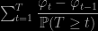
Heiko Strathman, Dino Sejdinovic and Mark Girolami have arXived a few weeks ago a paper on the use of a telescoping estimator to achieve an unbiased estimator of a Bayes estimator relying on the entire dataset, while using only a small proportion of the dataset. The idea is that a sequence  converging—to an unbiased estimator—of estimators φt can be turned into an unbiased estimator by a stopping rule T:

\sum_{t=1}^T \dfrac{\varphi_t-\varphi_{t-1}}{\mathbb{P}(T\ge t)}

is indeed unbiased. In a “Big Data” framework, the components φt are MCMC versions of posterior expectations based on a proportion αt of the data. And the stopping rule cannot exceed αt=1. The authors further propose to replicate this unbiased estimator R times on R parallel processors. They further claim a reduction in the computing cost of

\mathcal{O}(N^{1-\alpha})\qquad\text{if}\qquad\mathbb{P}(T=t)\approx e^{-\alpha t}

which means that a sub-linear cost can be achieved. However, the gain in computing time means higher variance than for the full MCMC solution:

“It is clear that running an MCMC chain on the full posterior, for any statistic, produces more accurate estimates than the debiasing approach, which by construction has an additional intrinsic source of variance. This means that if it is possible to produce even only a single MCMC sample (…), the resulting posterior expectation can be estimated with less expected error. It is therefore not instructive to compare approaches in that region. “

I first got a “free lunch” impression when reading the paper, namely it sounded like using a random stopping rule was enough to overcome unbiasedness and large size jams. This is not the message of the paper, but I remain both intrigued by the possibilities the unbiasedness offers and bemused by the claims therein, for several reasons: Continue reading →

amazing Gibbs sampler

Posted in Books, pictures, R, Statistics, University life with tags , , , , , , on February 19, 2015 by xi'an

BayesmWhen playing with Peter Rossi’s bayesm R package during a visit of Jean-Michel Marin to Paris, last week, we came up with the above Gibbs outcome. The setting is a Gaussian mixture model with three components in dimension 5 and the prior distributions are standard conjugate. In this case, with 500 observations and 5000 Gibbs iterations, the Markov chain (for one component of one mean of the mixture) has two highly distinct regimes: one that revolves around the true value of the parameter, 2.5, and one that explores a much broader area (which is associated with a much smaller value of the component weight). What we found amazing is the Gibbs ability to entertain both regimes, simultaneously.

testing MCMC code

Posted in Books, Statistics, University life with tags , , , , , , , , on December 26, 2014 by xi'an

Harvard2A title that caught my attention on arXiv: testing MCMC code by Roger Grosse and David Duvenaud. The paper is in fact a tutorial adapted from blog posts written by Grosse and Duvenaud, on the blog of the Harvard Intelligent Probabilistic Systems group. The purpose is to write code in such a modular way that (some) conditional probability computations can be tested. Using my favourite Gibbs sampler for the mixture model, they advocate computing the ratios

\dfrac{p(x'|z)}{p(x|z)}\quad\text{and}\quad \dfrac{p(x',z)}{p(x,z)}

to make sure they are exactly identical. (Where x denotes the part of the parameter being simulated and z anything else.) The paper also mentions an older paper by John Geweke—of which I was curiously unaware!—leading to another test: consider iterating the following two steps:

  1. update the parameter θ given the current data x by an MCMC step that preserves the posterior p(θ|x);
  2. update the data x given the current parameter value θ from the sampling distribution p(x|θ).

Since both steps preserve the joint distribution p(x,θ), values simulated from those steps should exhibit the same properties as a forward production of (x,θ), i.e., simulating from p(θ) and then from p(x|θ). So with enough simulations, comparison tests can be run. (Andrew has a very similar proposal at about the same time.) There are potential limitations to the first approach, obviously, from being unable to write the full conditionals [an ABC version anyone?!] to making a programming mistake that keep both ratios equal [as it would occur if a Metropolis-within-Gibbs was run by using the ratio of the joints in the acceptance probability]. Further, as noted by the authors it only addresses the mathematical correctness of the code, rather than the issue of whether the MCMC algorithm mixes well enough to provide a pseudo-iid-sample from p(θ|x). (Lack of mixing that could be spotted by Geweke’s test.) But it is so immediately available that it can indeed be added to every and all simulations involving a conditional step. While Geweke’s test requires re-running the MCMC algorithm altogether. Although clear divergence between an iid sampling from p(x,θ) and the Gibbs version above could appear fast enough for a stopping rule to be used. In fine, a worthwhile addition to the collection of checkings and tests built across the years for MCMC algorithms! (Of which the trick proposed by my friend Tobias Rydén to run first the MCMC code with n=0 observations in order to recover the prior p(θ) remains my favourite!)