 A question on Cross Validated led me to realise I had never truly considered the issue of periodic Gibbs samplers! In MCMC, non-aperiodic chains are a minor nuisance in that the skeleton trick of randomly subsampling the Markov chain leads to a aperiodic Markov chain. (The picture relates to the skeleton!) Intuitively, while the systematic Gibbs sampler has a tendency to non-reversibility, it seems difficult to imagine a sequence of full conditionals that would force the chain away from the current value..!In the discrete case, given that the current state of the Markov chain has positive probability for the target distribution, the conditional probabilities are all positive as well and hence the Markov chain can stay at its current value after one Gibbs cycle, with positive probabilities, which means strong aperiodicity. In the continuous case, a similar argument applies by considering a neighbourhood of the current value. (Incidentally, the same person asked a question about the absolute continuity of the Gibbs kernel. Being confused by our chapter on the topic!!!)
Archive for convergence
aperiodic Gibbs sampler
Posted in Books, Kids, pictures, Statistics, Travel, University life with tags aperiodicity, convergence, cross validated, Gibbs sampler, Markov chain, MCMC algorithms, Monte Carlo Statistical Methods, skeleton chain on February 11, 2015 by xi'anlabel switching in Bayesian mixture models
Posted in Books, Statistics, University life with tags component of a mixture, convergence, finite mixtures, identifiability, ill-posed problem, invariance, label switching, loss function, MCMC algorithms, missing data, multimodality, relabelling on October 31, 2014 by xi'an A referee of our paper on approximating evidence for mixture model with Jeong Eun Lee pointed out the recent paper by Carlos Rodríguez and Stephen Walker on label switching in Bayesian mixture models: deterministic relabelling strategies. Which appeared this year in JCGS and went beyond, below or above my radar.
Label switching is an issue with mixture estimation (and other latent variable models) because mixture models are ill-posed models where part of the parameter is not identifiable. Indeed, the density of a mixture being a sum of terms
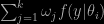
the parameter (vector) of the ω’s and of the θ’s is at best identifiable up to an arbitrary permutation of the components of the above sum. In other words, “component #1 of the mixture” is not a meaningful concept. And hence cannot be estimated.
This problem has been known for quite a while, much prior to EM and MCMC algorithms for mixtures, but it is only since mixtures have become truly estimable by Bayesian approaches that the debate has grown on this issue. In the very early days, Jean Diebolt and I proposed ordering the components in a unique way to give them a meaning. For instant, “component #1” would then be the component with the smallest mean or the smallest weight and so on… Later, in one of my favourite X papers, with Gilles Celeux and Merrilee Hurn, we exposed the convergence issues related with the non-identifiability of mixture models, namely that the posterior distributions were almost always multimodal, with a multiple of k! symmetric modes in the case of exchangeable priors, and therefore that Markov chains would have trouble to visit all those modes in a symmetric manner, despite the symmetry being guaranteed from the shape of the posterior. And we conclude with the slightly provocative statement that hardly any Markov chain inferring about mixture models had ever converged! In parallel, time-wise, Matthew Stephens had completed a thesis at Oxford on the same topic and proposed solutions for relabelling MCMC simulations in order to identify a single mode and hence produce meaningful estimators. Giving another meaning to the notion of “component #1”.
And then the topic began to attract more and more researchers, being both simple to describe and frustrating in its lack of definitive answer, both from simulation and inference perspectives. Rodriguez’s and Walker’s paper provides a survey on the label switching strategies in the Bayesian processing of mixtures, but its innovative part is in deriving a relabelling strategy. Which consists of finding the optimal permutation (at each iteration of the Markov chain) by minimising a loss function inspired from k-means clustering. Which is connected with both Stephens’ and our [JASA, 2000] loss functions. The performances of this new version are shown to be roughly comparable with those of other relabelling strategies, in the case of Gaussian mixtures. (Making me wonder if the choice of the loss function is not favourable to Gaussian mixtures.) And somehow faster than Stephens’ Kullback-Leibler loss approach.
“Hence, in an MCMC algorithm, the indices of the parameters can permute multiple times between iterations. As a result, we cannot identify the hidden groups that make [all] ergodic averages to estimate characteristics of the components useless.”
One section of the paper puzzles me, albeit it does not impact the methodology and the conclusions. In Section 2.1 (p.27), the authors consider the quantity

which is the marginal probability of allocating observation i to cluster or component j. Under an exchangeable prior, this quantity is uniformly equal to 1/k for all observations i and all components j, by virtue of the invariance under permutation of the indices… So at best this can serve as a control variate. Later in Section 2.2 (p.28), the above sentence does signal a problem with those averages but it seem to attribute it to MCMC behaviour rather than to the invariance of the posterior (or to the non-identifiability of the components per se). At last, the paper mentions that “given the allocations, the likelihood is invariant under permutations of the parameters and the allocations” (p.28), which is not correct, since eqn. (8)

does not hold when the two permutations σ and τ give different images of zi…
running MCMC for too long, and even longer…
Posted in Books, pictures, Running, Statistics, University life with tags ABC, acceptance rate, astronomy, astrostatistics, Bristol, convergence, Gibbs sampling, MCMC, Metropolis-Hastings algorithms, Monte Carlo Statistical Methods, simulated annealing, simulation on October 23, 2013 by xi'an Following my earlier post about the young astronomer who feared he was running his MCMC for too long, here is an update from his visit to my office this morning. This visit proved quite an instructive visit for both of us. (Disclaimer: the picture of an observatory seen from across Brunel’s suspension bridge in Bristol is as earlier completely unrelated with the young astronomer!)
First, the reason why he thought MCMC was running too long was that the acceptance rate was plummeting down to zero, whatever the random walk scale. The reason for this behaviour is that he was actually running a standard simulated annealing algorithm, hence observing the stabilisation of the Markov chain in one of the (global) modes of the target function. In that sense, he was right that the MCMC was run for “too long”, as there was nothing to expect once the mode had been reached and the temperature turned down to zero. So the algorithm was working correctly.
Second, the astronomy problem he considers had a rather complex likelihood, for which he substituted a distance between the (discretised) observed data and (discretised) simulated data, simulated conditional on the current parameter value. Now…does this ring a bell? If not, here is a three letter clue: ABC… Indeed, the trick he had found to get around this likelihood calculation issue was to re-invent a version of ABC-MCMC! Except that the distance was re-introduced into a regular MCMC scheme as a substitute to the log-likelihood. And compared with the distance at the previous MCMC iteration. This is quite clever, even though this substitution suffers from a normalisation issue (that I already mentioned in the post about Holmes’ and Walker’s idea to turn loss functions into pseudo likelihoods. Regular ABC does not encounter this difficult, obviously. I am still bemused by this reinvention of ABC from scratch!
So we are now at a stage where my young friend will experiment with (hopefully) correct ABC steps, trying to derive the tolerance value from warmup simulations and use some of the accelerating tricks suggested by Umberto Picchini and Julie Forman to avoid simulating the characteristics of millions of stars for nothing. And we agreed to meet soon for an update. Indeed, a fairly profitable morning for both of us!
running MCMC for too long…
Posted in Books, pictures, Running, Statistics, University life with tags acceptance rate, astronomy, Bristol, convergence, Gibbs sampling, MCMC, Metropolis-Hastings algorithms, Monte Carlo Statistical Methods, simulation on October 20, 2013 by xi'anHere is an excerpt from an email I just received from a young astronomer with whom I have had many email exchanges about the nature and implementation of MCMC algorithms, not making my point apparently:
The acceptance ratio turn to be good if I used (imposed by me) smaller numbers of iterations. What I think I am doing wrong is the convergence criteria. I am not stopping when I should stop.
To which I replied he should come (or Skype) and talk with me as I cannot get into enough details to point out his analysis is wrong… It may be the case that the MCMC algorithm finds a first mode, explores its neighbourhood (hence a good acceptance rate and green signals for convergence), then wanders away, attracted by other modes. It may also be the case the code has mistakes. Anyway, you cannot stop a (basic) MCMC algorithm too late or let it run for too long! (Disclaimer: the picture of an observatory seen from across Brunel’s suspension bridge in Bristol is unrelated to the young astronomer!)
Bayesian brittleness
Posted in Statistics with tags arXiv, Bayesian non-parametrics, convergence, inconsistent priors, mispecified model, Robins-Wasserman paradox on May 3, 2013 by xi'anHere is the abstract of a recently arXived paper that attracted my attention:
Although it is known that Bayesian estimators may be inconsistent if the model is misspecified, it is also a popular belief that a “good” or “close” enough model should have good convergence properties. This paper shows that, contrary to popular belief, there is no such thing as a “close enough” model in Bayesian inference in the following sense: we derive optimal lower and upper bounds on posterior values obtained from models that exactly capture an arbitrarily large number of finite-dimensional marginals of the data-generating distribution and/or that are arbitrarily close to the data-generating distribution in the Prokhorov or total variation metrics; these bounds show that such models may still make the largest possible prediction error after conditioning on an arbitrarily large number of sample data. Therefore, under model misspecification, and without stronger assumptions than (arbitrary) closeness in Prokhorov or total variation metrics, Bayesian inference offers no better guarantee of accuracy than arbitrarily picking a value between the essential infimum and supremum of the quantity of interest. In particular, an unscrupulous practitioner could slightly perturb a given prior and model to achieve any desired posterior conclusions.ink
The paper is both too long and too theoretical for me to get into it deep enough. The main point however is that, given the space of all possible measures, the set of (parametric) Bayes inferences constitutes a tiny finite-dimensional set that may lie far far away from the true model. I do not find the result unreasonable, far from it!, but the fact that Bayesian (and other) inferences may be inconsistent for most misspecified models is not such a major issue in my opinion. (Witness my post on the Robins-Wasserman paradox.) I am not so much convinced either about this “popular belief that a “good” or “close” enough model should have good convergence properties”, as it is intuitively reasonable that the immensity of the space of all models can induce non-convergent behaviours. The statistical question is rather what can be done about it. Does it matter that the model is misspecified? If it does, is there any meaning in estimating parameters without a model? For a finite sample size, should we at all bother that the model is not “right” or “close enough” if discrepancies cannot be detected at this precision level? I think the answer to all those questions is negative and that we should proceed with our imperfect models and imperfect inference as long as our imperfect simulation tools do not exhibit strong divergences.


