puzzle | Xi'an's Og

Archive for puzzle

R puzzle

Posted in Statistics with tags codegolf, puzzle, R on September 12, 2019 by xi'an

Can you guess the meaning of the following R code

"?"=`u\164f8ToI\x6Et`;'!'=prod;!{
    y<-xtabs(~?readLines())}%in%{
     z<-y[1]}&z>T##&[]>~48bEfILpu

If not (!), the explanation is provided in Robin’s answer to a codegolf puzzle.

who’s that travelling salesman path?!

Posted in Statistics with tags image processing, puzzle, StippleGen, travelling salesman on July 18, 2017 by xi'an

2 Comments »

Asher’s enigma

Posted in R, Statistics with tags beta distribution, puzzle, R-bloggers, unit square on July 26, 2010 by xi'an

On his Probability and statistics blog, Matt Asher put a funny question (with my rephrasing):

Take a unit square. Now pick two spots at random along the perimeter, uniformly. For each of these two locations, pick another random point from one of the three other sides of the square and draw the segment. What is the probability the two segments intersect? And what is the distribution for the intersection points?

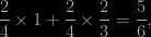
The (my) intuition for the first question was 1/2, but a quick computation led to another answer. The key to the computation is to distinguish whether or not both segments share one side of the square. They do with probability

$\dfrac{2}{4}\times 1 + \dfrac{2}{4}\times\dfrac{2}{3} = \dfrac{5}{6},$

in which case they intersect with probability 1/2. They occupy the four sides with probability 1/6, in which case they intersect with probability 1/3. So the final answer is 17/36 (as posted by several readers and empirically found by Matt). The second question is much more tricky: the histogram of the distribution of the coordinates is peaked towards the boundaries, thus reminding me of an arc-sine distribution, but there is a bump in the middle as well. Computing the coordinates of the intersection depending on the respective positions of the endpoints of both segments and simulating those distributions led me to histograms that looked either like beta B(a,a) distributions, or like beta B(1,a) distributions, or like beta B(a,1) distributions… Not exactly, though. So not even a mixture of beta distributions is enough to explain the distribution of the intersection points… For instance, the intersection points corresponding to segments were both segments start from the same side and end up in the opposite side are distributed as

$\dfrac{u_1(u_4-u_3)-u_3(u_2-u_1)}{u_4-u_3-u_2+u_1}$

where all u‘s are uniform on (0,1) and under the constraint $(u_2-u_1)(u_4-u_3)<0$ . The following graph shows how well a beta distribution fits in that case. (Not perfectly, though!)
The R code is

u=matrix(runif(4*10^5),ncol=4)
u[,c(1,3)]=t(apply(u[,c(1,3)],1,sort))
u[,c(2,4)]=-t(apply(-u[,c(2,4)],1,sort))
y=(u[,1]*(u[,4]-u[,3])-u[,3]*(u[,2]-u[,1]))/(u[,1]+u[,4]-u[,2]-u[,3])

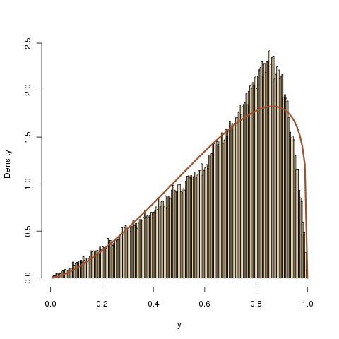
Similarly, if the two segments start from the same side but end up on different sides, the distribution of one coordinate is given by

$\dfrac{u_1(1-u_3)-u_3u_4(u_2-u_1)}{1-u_3-u_4(u_2-u_1)}$

under the constraint $u_3<u_1$ . The outcome is once again almost distributed as a beta:
The corresponding R code is

u=matrix(runif(4*10^5),ncol=4)
u[,c(1,3)]=-t(apply(-u[,c(1,3)],1,sort))
y=(u[,1]*(1-u[,3])-u[,3]*u[,4]*(u[,2]-u[,1]))/(1-u[,3]-u[,4]*(u[,2]-u[,1]))

Le Monde rank test (corr’d)

Posted in R, Statistics with tags Le Monde, puzzle, R, Spearman rank test on April 7, 2010 by xi'an

Since my first representation of the rank statistic as paired was incorrect, here is the histogram produced by the simulation

perm=sample(1:20)
saple[t]=sum(abs(sort(perm[1:10])-sort(perm[11:20])))

when $n=20$ . It is obviously much closer to zero than previously.

An interesting change is that the regression of the log-mean on $log(n)$ produces

> lm(log(memean)~log(enn))
Call:
lm(formula = log(memean) ~ log(enn))
Coefficients:
(Intercept)     log(enn)
 -1.162        1.499

meaning that the mean is in $n^{3/2}$ rather than in $n$ or $n^2$ :

> summary(lm(memean~eth-1))
Coefficients:
      Estimate Std. Error t value Pr(>|t|)
eth 0.3117990  0.0002719    1147   <2e-16 ***

with a very good fit.

1 Comment »

Le Monde rank test

Posted in R, Statistics with tags climate change, climatosceptic, correlation, global warming, Le Monde, puzzle, R, Robin Ryder, Spearman rank test on April 5, 2010 by xi'an

In the puzzle found in Le Monde of this weekend, the mathematical object behind the silly story is defined as a pseudo-Spearman rank correlation test statistic,

$\mathfrak{M}_n = \sum_{i=1}^n |r^x_i-r^y_i|\,,$

where the difference between the ranks of the paired random variables $x_i$ and $y_i$ is in absolute value instead of being squared as in the Spearman rank test statistic. I don’t know whether or not this measure of distance has been studied in the statistics literature (although I’d be surprised has it not been studied!). Here is an histogram of the distribution of the new statistics for $n=20$ under the null hypothesis that both samples are uncorrelated (i.e. that the sequence of ranks is a random permutation). Each point in the sample was obtained by

perm=sample(1:20)
saple[t]=sum(abs(perm[1:10]-perm[11:20]))

When regressing the mean of this statistic $\mathfrak{M}_n$ against the covariates $n$ and $n^2$ , I obtain the uninspiring formula

$\mathbb{E} [\mathfrak{M}_n] \approx 0.1681 n^2 - 0.3769 n + 11.1921$

which does not translate into a nice polynomial in $n$ !

Another interesting probabilistic/combinatorial problem issued from an earlier Le Monde puzzle: given an urn with $n$ white balls and $n$ black balls that is sampled without replacement, what is the probability that there exists a sequence of length $2k$ with the same number of white and black balls for $k=1,\ldots,n$ ? If $k=1,n$ , the answer is obviously one (1), but for some values of $k$ , it is less than one. When $n$ goes to infinity, this is somehow related to the probability that a Brownian bridge crosses the axis in-between $0$ and $1$ but I have no clue whether this helps or not! Robin Ryder solved the question for the values $n=50$ and $k=24,25$ by establishing that the probability is still one.

Ps- The same math tribune in Le Monde coincidently advertises a book, Le Mythe Climatique, by Benoît Rittaud that adresses … climate change issues and the “statistical mistakes made by climatologists”. The interesting point (if any) is that Benoît Rittaud is a “mathematician not a statistician”, with a few papers in ergodic theory, but this advocated climatoskeptic nonetheless criticises the use of both statistical and simulation tools in climate modeling. (“Simulation has only been around for a few dozen years, a very short span in the history of sciences. The climate debate may be an opportunity to reassess the role of simulation in the scientific process.”)

2 Comments »

	David on Bayesian workflow [book review…
	Ewan on Tidy up, Claude!
	xi'an on Tidy up, Claude!
	Ewan on Tidy up, Claude!
	Ewan on Já við viðræðum. Já við Evrópu…

Xi'an's Og

Archive for puzzle

R puzzle

Like this:

who’s that travelling salesman path?!

Like this:

Asher’s enigma

Like this:

Le Monde rank test (corr’d)

Like this:

Le Monde rank test

Like this:

blogs & links

Recent entries

Latest comments

Og\’s RSS

Xi'an's Og

Archive for puzzle

R puzzle

Share:

Like this:

who’s that travelling salesman path?!

Share:

Like this:

Asher’s enigma

Share:

Like this:

Le Monde rank test (corr’d)

Share:

Like this:

Le Monde rank test

Share:

Like this:

blogs & links

Tags

Recent entries

Latest comments

Og\’s RSS